Wick-to-Body Ratio Trend Forecast | Flux ChartsThe Wick-to-Body Ratio Trend Forecast Indicator aims to forecast potential movements following the last closed candle using the wick-to-body ratio. The script identifies those candles within the loopback period with a ratio matching that of the last closed candle and provides an analysis of their trends.
➡️ USAGE
Wick-to-body ratios can be used in many strategies. The most common use in stock trading is to discern bullish or bearish sentiment. This indicator extends candle ratios, revealing previous patterns that follow a candle with a similar ratio. The most basic use of this indicator is the single forecast line.
➡️ FORECASTING SYSTEM
This line displays a compilation of the averages of all the previous trends resulting from those historical candles with a matching ratio. It shows the average movements of the trends as well as the 'strength' of the trend. The 'strength' of the trend is a gradient that is blue when the trend deviates more from the average and red when it deviates less.
Chart: AMEX:SPY 30 min; Indicator Settings: Loopback 700, Previous Trends ON
The color-coded deviation is visible in this image of the indicator with the default settings (except for Forecast Lines > Previous Trends ), and the trend line grows bluer as the past patterns deviate more.
➡️ ADAPTIVE ACCEPTABLE RANGE
The algorithm looks back at every candle within the loopback period to find candles that match the last closed candle. The algorithm adaptively changes the acceptable range to which a candle can differ from the ratio of the last closed candle. The algorithm will never have more than 15 historical points used, as it will lower its sensitivity before it reaches that point.
Chart: BITSTAMP:BTCUSD 5 min; Indicator Settings: Loopback 700
Here is the BTC chart on 7/6/23 with default settings except for the loopback period at 700.
Chart: BITSTAMP:BTCUSD 5 min; Indicator Settings: Loopback 200
Here is the exact same chart with a loopback period of 200. While the first ratio for both is the same, a new ratio is revealed for the chart with a loopback of only 200 because the adaptive range is adjusted in the algorithm to find an acceptable number of reference points. Note the table in the top right however, while the algorithm adapts the acceptable range between the current ratio and historical ones to find reference points, there is a threshold at which candles will be considered too inaccurate to be considered. This prevents meaningless associations between candles due to a particularly rare ratio. This threshold can be adjusted in the settings through "Default Accuracy".
Machinelearning
RSI-MFI Machine Learning [ Manhattan distance ]The RSI-MFI Machine Learning Indicator is a technical analysis tool that combines the Relative Strength Index (RSI) and Money Flow Index (MFI) indicators with the Manhattan distance metric.
It aims to provide insights into potential trade setups by leveraging machine learning principles and calculating distances between current and historical data points.
The indicator starts by calculating the RSI and MFI values based on the specified periods for each indicator.
The RSI measures the strength and speed of price movements, while the MFI evaluates the inflow and outflow of money in the market.
By combining these two indicators, the indicator captures both price momentum and money flow dynamics.
To apply machine learning principles , the indicator utilizes the Manhattan distance metric to quantify the similarity or dissimilarity between different data points.
The Manhattan distance is calculated by taking the absolute differences between corresponding RSI and MFI values of the current point and historical points.
Next, the indicator determines the nearest neighbors based on the calculated Manhattan distances.
The number of nearest neighbors is determined by the square root of the specified count of neighbors.
By identifying similar patterns and behaviors in the historical data, the indicator aims to uncover potential trade opportunities.
Trade signals are generated based on the calculated distances. The indicator compares each distance with the maximum distance encountered so far.
If a new maximum distance is found, it updates the value and considers the corresponding direction as a potential trade signal. The trade signals are stored in an array for further analysis.
Furthermore, the indicator considers the price action and a calculated regression line to differentiate between long and short trade signals.
Long trade signals are identified when the closing price is above the regression line, indicating a potentially bullish setup.
Short trade signals are identified when the closing price is below the regression line, indicating a potentially bearish setup.
The RSI-MFI Machine Learning Indicator visualizes the regression line on the price chart and labels the bars accordingly. It highlights the regression line with different colors based on the trade signals, making it easier for traders to identify potential entry or exit points.
Traders can use the RSI-MFI Machine Learning Indicator as a tool to analyze price movements, evaluate market conditions based on RSI and MFI, leverage machine learning concepts to find similar patterns, and make informed trading decisions.
Machine Learning : Torben's Moving Median KNN BandsWhat is Median Filtering ?
Median filtering is a non-linear digital filtering technique, often used to remove noise from an image or signal. Such noise reduction is a typical pre-processing step to improve the results of later processing (for example, edge detection on an image). Median filtering is very widely used in digital image processing because, under certain conditions, it preserves edges while removing noise (but see the discussion below), also having applications in signal processing.
The main idea of the median filter is to run through the signal entry by entry, replacing each entry with the median of neighboring entries. The pattern of neighbors is called the "window", which slides, entry by entry, over the entire signal. For one-dimensional signals, the most obvious window is just the first few preceding and following entries, whereas for two-dimensional (or higher-dimensional) data the window must include all entries within a given radius or ellipsoidal region (i.e. the median filter is not a separable filter).
The median filter works by taking the median of all the pixels in a neighborhood around the current pixel. The median is the middle value in a sorted list of numbers. This means that the median filter is not sensitive to the order of the pixels in the neighborhood, and it is not affected by outliers (very high or very low values).
The median filter is a very effective way to remove noise from images. It can remove both salt and pepper noise (random white and black pixels) and Gaussian noise (randomly distributed pixels with a Gaussian distribution). The median filter is also very good at preserving edges, which is why it is often used as a pre-processing step for edge detection.
However, the median filter can also blur images. This is because the median filter replaces each pixel with the value of the median of its neighbors. This can cause the edges of objects in the image to be smoothed out. The amount of blurring depends on the size of the window used by the median filter. A larger window will blur more than a smaller window.
The median filter is a very versatile tool that can be used for a variety of tasks in image processing. It is a good choice for removing noise and preserving edges, but it can also blur images. The best way to use the median filter is to experiment with different window sizes to find the setting that produces the desired results.
What is this Indicator ?
K-nearest neighbors (KNN) is a simple, non-parametric machine learning algorithm that can be used for both classification and regression tasks. The basic idea behind KNN is to find the K most similar data points to a new data point and then use the labels of those K data points to predict the label of the new data point.
Torben's moving median is a variation of the median filter that is used to remove noise from images. The median filter works by replacing each pixel in an image with the median of its neighbors. Torben's moving median works in a similar way, but it also averages the values of the neighbors. This helps to reduce the amount of blurring that can occur with the median filter.
KNN over Torben's moving median is a hybrid algorithm that combines the strengths of both KNN and Torben's moving median. KNN is able to learn the underlying distribution of the data, while Torben's moving median is able to remove noise from the data. This combination can lead to better performance than either algorithm on its own.
To implement KNN over Torben's moving median, we first need to choose a value for K. The value of K controls how many neighbors are used to predict the label of a new data point. A larger value of K will make the algorithm more robust to noise, but it will also make the algorithm less sensitive to local variations in the data.
Once we have chosen a value for K, we need to train the algorithm on a dataset of labeled data points. The training dataset will be used to learn the underlying distribution of the data.
Once the algorithm is trained, we can use it to predict the labels of new data points. To do this, we first need to find the K most similar data points to the new data point. We can then use the labels of those K data points to predict the label of the new data point.
KNN over Torben's moving median is a simple, yet powerful algorithm that can be used for a variety of tasks. It is particularly well-suited for tasks where the data is noisy or where the underlying distribution of the data is unknown.
Here are some of the advantages of using KNN over Torben's moving median:
KNN is able to learn the underlying distribution of the data.
KNN is robust to noise.
KNN is not sensitive to local variations in the data.
Here are some of the disadvantages of using KNN over Torben's moving median:
KNN can be computationally expensive for large datasets.
KNN can be sensitive to the choice of K.
KNN can be slow to train.

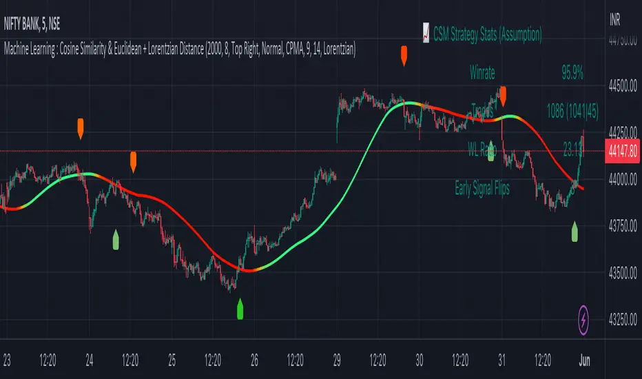
Machine Learning : Cosine Similarity & Euclidean DistanceIntroduction:
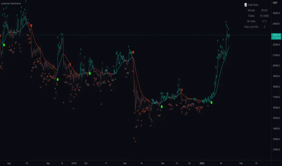
This script implements a comprehensive trading strategy that adheres to the established rules and guidelines of housing trading. It leverages advanced machine learning techniques and incorporates customised moving averages, including the Conceptive Price Moving Average (CPMA), to provide accurate signals for informed trading decisions in the housing market. Additionally, signal processing techniques such as Lorentzian, Euclidean distance, Cosine similarity, Know sure thing, Rational Quadratic, and sigmoid transformation are utilised to enhance the signal quality and improve trading accuracy.
Features:
Market Analysis: The script utilizes advanced machine learning methods such as Lorentzian, Euclidean distance, and Cosine similarity to analyse market conditions. These techniques measure the similarity and distance between data points, enabling more precise signal identification and enhancing trading decisions.
Cosine similarity:
Cosine similarity is a measure used to determine the similarity between two vectors, typically in a high-dimensional space. It calculates the cosine of the angle between the vectors, indicating the degree of similarity or dissimilarity.
In the context of trading or signal processing, cosine similarity can be employed to compare the similarity between different data points or signals. The vectors in this case represent the numerical representations of the data points or signals.
Cosine similarity ranges from -1 to 1, with 1 indicating perfect similarity, 0 indicating no similarity, and -1 indicating perfect dissimilarity. A higher cosine similarity value suggests a closer match between the vectors, implying that the signals or data points share similar characteristics.
Lorentzian Classification:
Lorentzian classification is a machine learning algorithm used for classification tasks. It is based on the Lorentzian distance metric, which measures the similarity or dissimilarity between two data points. The Lorentzian distance takes into account the shape of the data distribution and can handle outliers better than other distance metrics.
Euclidean Distance:
Euclidean distance is a distance metric widely used in mathematics and machine learning. It calculates the straight-line distance between two points in Euclidean space. In two-dimensional space, the Euclidean distance between two points (x1, y1) and (x2, y2) is calculated using the formula sqrt((x2 - x1)^2 + (y2 - y1)^2).
Dynamic Time Windows: The script incorporates a dynamic time window function that allows users to define specific time ranges for trading. It checks if the current time falls within the specified window to execute the relevant trading signals.
Custom Moving Averages: The script includes the CPMA, a powerful moving average calculation. Unlike traditional moving averages, the CPMA provides improved support and resistance levels by considering multiple price types and employing a combination of Exponential Moving Averages (EMAs) and Simple Moving Averages (SMAs). Its adaptive nature ensures responsiveness to changes in price trends.
Signal Processing Techniques: The script applies signal processing techniques such as Know sure thing, Rational Quadratic, and sigmoid transformation to enhance the quality of the generated signals. These techniques improve the accuracy and reliability of the trading signals, aiding in making well-informed trading decisions.
Trade Statistics and Metrics: The script provides comprehensive trade statistics and metrics, including total wins, losses, win rate, win-loss ratio, and early signal flips. These metrics offer valuable insights into the performance and effectiveness of the trading strategy.
Usage:
Configuring Time Windows: Users can customize the time windows by specifying the start and finish time ranges according to their trading preferences and local market conditions.
Signal Interpretation: The script generates long and short signals based on the analysis, custom moving averages, and signal processing techniques. Users should pay attention to these signals and take appropriate action, such as entering or exiting trades, depending on their trading strategies.
Trade Statistics: The script continuously tracks and updates trade statistics, providing users with a clear overview of their trading performance. These statistics help users assess the effectiveness of the strategy and make informed decisions.
Conclusion:
With its adherence to housing trading rules, advanced machine learning methods, customized moving averages like the CPMA, and signal processing techniques such as Lorentzian, Euclidean distance, Cosine similarity, Know sure thing, Rational Quadratic, and sigmoid transformation, this script offers users a powerful tool for housing market analysis and trading. By leveraging the provided signals, time windows, and trade statistics, users can enhance their trading strategies and improve their overall trading performance.
Disclaimer:
Please note that while this script incorporates established tradingview housing rules, advanced machine learning techniques, customized moving averages, and signal processing techniques, it should be used for informational purposes only. Users are advised to conduct their own analysis and exercise caution when making trading decisions. The script's performance may vary based on market conditions, user settings, and the accuracy of the machine learning methods and signal processing techniques. The trading platform and developers are not responsible for any financial losses incurred while using this script.
By publishing this script on the platform, traders can benefit from its professional presentation, clear instructions, and the utilisation of advanced machine learning techniques, customised moving averages, and signal processing techniques for enhanced trading signals and accuracy.
I extend my gratitude to TradingView, LUX ALGO, and JDEHORTY for their invaluable contributions to the trading community. Their innovative scripts, meticulous coding patterns, and insightful ideas have profoundly enriched traders' strategies, including my own.
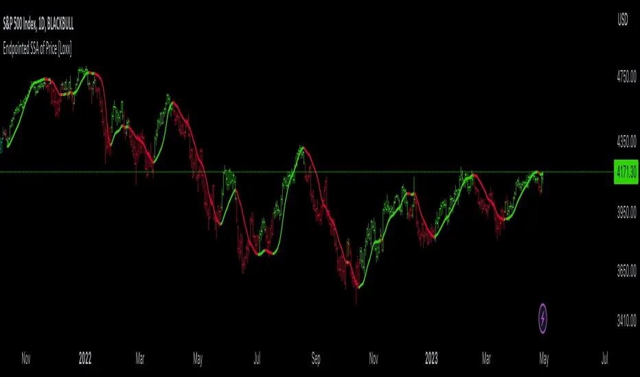
Endpointed SSA of Price [Loxx]The Endpointed SSA of Price: A Comprehensive Tool for Market Analysis and Decision-Making
The financial markets present sophisticated challenges for traders and investors as they navigate the complexities of market behavior. To effectively interpret and capitalize on these complexities, it is crucial to employ powerful analytical tools that can reveal hidden patterns and trends. One such tool is the Endpointed SSA of Price, which combines the strengths of Caterpillar Singular Spectrum Analysis, a sophisticated time series decomposition method, with insights from the fields of economics, artificial intelligence, and machine learning.
The Endpointed SSA of Price has its roots in the interdisciplinary fusion of mathematical techniques, economic understanding, and advancements in artificial intelligence. This unique combination allows for a versatile and reliable tool that can aid traders and investors in making informed decisions based on comprehensive market analysis.
The Endpointed SSA of Price is not only valuable for experienced traders but also serves as a useful resource for those new to the financial markets. By providing a deeper understanding of market forces, this innovative indicator equips users with the knowledge and confidence to better assess risks and opportunities in their financial pursuits.
█ Exploring Caterpillar SSA: Applications in AI, Machine Learning, and Finance
Caterpillar SSA (Singular Spectrum Analysis) is a non-parametric method for time series analysis and signal processing. It is based on a combination of principles from classical time series analysis, multivariate statistics, and the theory of random processes. The method was initially developed in the early 1990s by a group of Russian mathematicians, including Golyandina, Nekrutkin, and Zhigljavsky.
Background Information:
SSA is an advanced technique for decomposing time series data into a sum of interpretable components, such as trend, seasonality, and noise. This decomposition allows for a better understanding of the underlying structure of the data and facilitates forecasting, smoothing, and anomaly detection. Caterpillar SSA is a particular implementation of SSA that has proven to be computationally efficient and effective for handling large datasets.
Uses in AI and Machine Learning:
In recent years, Caterpillar SSA has found applications in various fields of artificial intelligence (AI) and machine learning. Some of these applications include:
1. Feature extraction: Caterpillar SSA can be used to extract meaningful features from time series data, which can then serve as inputs for machine learning models. These features can help improve the performance of various models, such as regression, classification, and clustering algorithms.
2. Dimensionality reduction: Caterpillar SSA can be employed as a dimensionality reduction technique, similar to Principal Component Analysis (PCA). It helps identify the most significant components of a high-dimensional dataset, reducing the computational complexity and mitigating the "curse of dimensionality" in machine learning tasks.
3. Anomaly detection: The decomposition of a time series into interpretable components through Caterpillar SSA can help in identifying unusual patterns or outliers in the data. Machine learning models trained on these decomposed components can detect anomalies more effectively, as the noise component is separated from the signal.
4. Forecasting: Caterpillar SSA has been used in combination with machine learning techniques, such as neural networks, to improve forecasting accuracy. By decomposing a time series into its underlying components, machine learning models can better capture the trends and seasonality in the data, resulting in more accurate predictions.
Application in Financial Markets and Economics:
Caterpillar SSA has been employed in various domains within financial markets and economics. Some notable applications include:
1. Stock price analysis: Caterpillar SSA can be used to analyze and forecast stock prices by decomposing them into trend, seasonal, and noise components. This decomposition can help traders and investors better understand market dynamics, detect potential turning points, and make more informed decisions.
2. Economic indicators: Caterpillar SSA has been used to analyze and forecast economic indicators, such as GDP, inflation, and unemployment rates. By decomposing these time series, researchers can better understand the underlying factors driving economic fluctuations and develop more accurate forecasting models.
3. Portfolio optimization: By applying Caterpillar SSA to financial time series data, portfolio managers can better understand the relationships between different assets and make more informed decisions regarding asset allocation and risk management.
Application in the Indicator:
In the given indicator, Caterpillar SSA is applied to a financial time series (price data) to smooth the series and detect significant trends or turning points. The method is used to decompose the price data into a set number of components, which are then combined to generate a smoothed signal. This signal can help traders and investors identify potential entry and exit points for their trades.
The indicator applies the Caterpillar SSA method by first constructing the trajectory matrix using the price data, then computing the singular value decomposition (SVD) of the matrix, and finally reconstructing the time series using a selected number of components. The reconstructed series serves as a smoothed version of the original price data, highlighting significant trends and turning points. The indicator can be customized by adjusting the lag, number of computations, and number of components used in the reconstruction process. By fine-tuning these parameters, traders and investors can optimize the indicator to better match their specific trading style and risk tolerance.
Caterpillar SSA is versatile and can be applied to various types of financial instruments, such as stocks, bonds, commodities, and currencies. It can also be combined with other technical analysis tools or indicators to create a comprehensive trading system. For example, a trader might use Caterpillar SSA to identify the primary trend in a market and then employ additional indicators, such as moving averages or RSI, to confirm the trend and generate trading signals.
In summary, Caterpillar SSA is a powerful time series analysis technique that has found applications in AI and machine learning, as well as financial markets and economics. By decomposing a time series into interpretable components, Caterpillar SSA enables better understanding of the underlying structure of the data, facilitating forecasting, smoothing, and anomaly detection. In the context of financial trading, the technique is used to analyze price data, detect significant trends or turning points, and inform trading decisions.
█ Input Parameters
This indicator takes several inputs that affect its signal output. These inputs can be classified into three categories: Basic Settings, UI Options, and Computation Parameters.
Source: This input represents the source of price data, which is typically the closing price of an asset. The user can select other price data, such as opening price, high price, or low price. The selected price data is then utilized in the Caterpillar SSA calculation process.
Lag: The lag input determines the window size used for the time series decomposition. A higher lag value implies that the SSA algorithm will consider a longer range of historical data when extracting the underlying trend and components. This parameter is crucial, as it directly impacts the resulting smoothed series and the quality of extracted components.
Number of Computations: This input, denoted as 'ncomp,' specifies the number of eigencomponents to be considered in the reconstruction of the time series. A smaller value results in a smoother output signal, while a higher value retains more details in the series, potentially capturing short-term fluctuations.
SSA Period Normalization: This input is used to normalize the SSA period, which adjusts the significance of each eigencomponent to the overall signal. It helps in making the algorithm adaptive to different timeframes and market conditions.
Number of Bars: This input specifies the number of bars to be processed by the algorithm. It controls the range of data used for calculations and directly affects the computation time and the output signal.
Number of Bars to Render: This input sets the number of bars to be plotted on the chart. A higher value slows down the computation but provides a more comprehensive view of the indicator's performance over a longer period. This value controls how far back the indicator is rendered.
Color bars: This boolean input determines whether the bars should be colored according to the signal's direction. If set to true, the bars are colored using the defined colors, which visually indicate the trend direction.
Show signals: This boolean input controls the display of buy and sell signals on the chart. If set to true, the indicator plots shapes (triangles) to represent long and short trade signals.
Static Computation Parameters:
The indicator also includes several internal parameters that affect the Caterpillar SSA algorithm, such as Maxncomp, MaxLag, and MaxArrayLength. These parameters set the maximum allowed values for the number of computations, the lag, and the array length, ensuring that the calculations remain within reasonable limits and do not consume excessive computational resources.
█ A Note on Endpionted, Non-repainting Indicators
An endpointed indicator is one that does not recalculate or repaint its past values based on new incoming data. In other words, the indicator's previous signals remain the same even as new price data is added. This is an important feature because it ensures that the signals generated by the indicator are reliable and accurate, even after the fact.
When an indicator is non-repainting or endpointed, it means that the trader can have confidence in the signals being generated, knowing that they will not change as new data comes in. This allows traders to make informed decisions based on historical signals, without the fear of the signals being invalidated in the future.
In the case of the Endpointed SSA of Price, this non-repainting property is particularly valuable because it allows traders to identify trend changes and reversals with a high degree of accuracy, which can be used to inform trading decisions. This can be especially important in volatile markets where quick decisions need to be made.
Machine Learning: Lorentzian Classification█ OVERVIEW
A Lorentzian Distance Classifier (LDC) is a Machine Learning classification algorithm capable of categorizing historical data from a multi-dimensional feature space. This indicator demonstrates how Lorentzian Classification can also be used to predict the direction of future price movements when used as the distance metric for a novel implementation of an Approximate Nearest Neighbors (ANN) algorithm.
█ BACKGROUND
In physics, Lorentzian space is perhaps best known for its role in describing the curvature of space-time in Einstein's theory of General Relativity (2). Interestingly, however, this abstract concept from theoretical physics also has tangible real-world applications in trading.
Recently, it was hypothesized that Lorentzian space was also well-suited for analyzing time-series data (4), (5). This hypothesis has been supported by several empirical studies that demonstrate that Lorentzian distance is more robust to outliers and noise than the more commonly used Euclidean distance (1), (3), (6). Furthermore, Lorentzian distance was also shown to outperform dozens of other highly regarded distance metrics, including Manhattan distance, Bhattacharyya similarity, and Cosine similarity (1), (3). Outside of Dynamic Time Warping based approaches, which are unfortunately too computationally intensive for PineScript at this time, the Lorentzian Distance metric consistently scores the highest mean accuracy over a wide variety of time series data sets (1).
Euclidean distance is commonly used as the default distance metric for NN-based search algorithms, but it may not always be the best choice when dealing with financial market data. This is because financial market data can be significantly impacted by proximity to major world events such as FOMC Meetings and Black Swan events. This event-based distortion of market data can be framed as similar to the gravitational warping caused by a massive object on the space-time continuum. For financial markets, the analogous continuum that experiences warping can be referred to as "price-time".
Below is a side-by-side comparison of how neighborhoods of similar historical points appear in three-dimensional Euclidean Space and Lorentzian Space:
This figure demonstrates how Lorentzian space can better accommodate the warping of price-time since the Lorentzian distance function compresses the Euclidean neighborhood in such a way that the new neighborhood distribution in Lorentzian space tends to cluster around each of the major feature axes in addition to the origin itself. This means that, even though some nearest neighbors will be the same regardless of the distance metric used, Lorentzian space will also allow for the consideration of historical points that would otherwise never be considered with a Euclidean distance metric.
Intuitively, the advantage inherent in the Lorentzian distance metric makes sense. For example, it is logical that the price action that occurs in the hours after Chairman Powell finishes delivering a speech would resemble at least some of the previous times when he finished delivering a speech. This may be true regardless of other factors, such as whether or not the market was overbought or oversold at the time or if the macro conditions were more bullish or bearish overall. These historical reference points are extremely valuable for predictive models, yet the Euclidean distance metric would miss these neighbors entirely, often in favor of irrelevant data points from the day before the event. By using Lorentzian distance as a metric, the ML model is instead able to consider the warping of price-time caused by the event and, ultimately, transcend the temporal bias imposed on it by the time series.
For more information on the implementation details of the Approximate Nearest Neighbors (ANN) algorithm used in this indicator, please refer to the detailed comments in the source code.
█ HOW TO USE
Below is an explanatory breakdown of the different parts of this indicator as it appears in the interface:
Below is an explanation of the different settings for this indicator:
General Settings:
Source - This has a default value of "hlc3" and is used to control the input data source.
Neighbors Count - This has a default value of 8, a minimum value of 1, a maximum value of 100, and a step of 1. It is used to control the number of neighbors to consider.
Max Bars Back - This has a default value of 2000.
Feature Count - This has a default value of 5, a minimum value of 2, and a maximum value of 5. It controls the number of features to use for ML predictions.
Color Compression - This has a default value of 1, a minimum value of 1, and a maximum value of 10. It is used to control the compression factor for adjusting the intensity of the color scale.
Show Exits - This has a default value of false. It controls whether to show the exit threshold on the chart.
Use Dynamic Exits - This has a default value of false. It is used to control whether to attempt to let profits ride by dynamically adjusting the exit threshold based on kernel regression.
Feature Engineering Settings:
Note: The Feature Engineering section is for fine-tuning the features used for ML predictions. The default values are optimized for the 4H to 12H timeframes for most charts, but they should also work reasonably well for other timeframes. By default, the model can support features that accept two parameters (Parameter A and Parameter B, respectively). Even though there are only 4 features provided by default, the same feature with different settings counts as two separate features. If the feature only accepts one parameter, then the second parameter will default to EMA-based smoothing with a default value of 1. These features represent the most effective combination I have encountered in my testing, but additional features may be added as additional options in the future.
Feature 1 - This has a default value of "RSI" and options are: "RSI", "WT", "CCI", "ADX".
Feature 2 - This has a default value of "WT" and options are: "RSI", "WT", "CCI", "ADX".
Feature 3 - This has a default value of "CCI" and options are: "RSI", "WT", "CCI", "ADX".
Feature 4 - This has a default value of "ADX" and options are: "RSI", "WT", "CCI", "ADX".
Feature 5 - This has a default value of "RSI" and options are: "RSI", "WT", "CCI", "ADX".
Filters Settings:
Use Volatility Filter - This has a default value of true. It is used to control whether to use the volatility filter.
Use Regime Filter - This has a default value of true. It is used to control whether to use the trend detection filter.
Use ADX Filter - This has a default value of false. It is used to control whether to use the ADX filter.
Regime Threshold - This has a default value of -0.1, a minimum value of -10, a maximum value of 10, and a step of 0.1. It is used to control the Regime Detection filter for detecting Trending/Ranging markets.
ADX Threshold - This has a default value of 20, a minimum value of 0, a maximum value of 100, and a step of 1. It is used to control the threshold for detecting Trending/Ranging markets.
Kernel Regression Settings:
Trade with Kernel - This has a default value of true. It is used to control whether to trade with the kernel.
Show Kernel Estimate - This has a default value of true. It is used to control whether to show the kernel estimate.
Lookback Window - This has a default value of 8 and a minimum value of 3. It is used to control the number of bars used for the estimation. Recommended range: 3-50
Relative Weighting - This has a default value of 8 and a step size of 0.25. It is used to control the relative weighting of time frames. Recommended range: 0.25-25
Start Regression at Bar - This has a default value of 25. It is used to control the bar index on which to start regression. Recommended range: 0-25
Display Settings:
Show Bar Colors - This has a default value of true. It is used to control whether to show the bar colors.
Show Bar Prediction Values - This has a default value of true. It controls whether to show the ML model's evaluation of each bar as an integer.
Use ATR Offset - This has a default value of false. It controls whether to use the ATR offset instead of the bar prediction offset.
Bar Prediction Offset - This has a default value of 0 and a minimum value of 0. It is used to control the offset of the bar predictions as a percentage from the bar high or close.
Backtesting Settings:
Show Backtest Results - This has a default value of true. It is used to control whether to display the win rate of the given configuration.
█ WORKS CITED
(1) R. Giusti and G. E. A. P. A. Batista, "An Empirical Comparison of Dissimilarity Measures for Time Series Classification," 2013 Brazilian Conference on Intelligent Systems, Oct. 2013, DOI: 10.1109/bracis.2013.22.
(2) Y. Kerimbekov, H. Ş. Bilge, and H. H. Uğurlu, "The use of Lorentzian distance metric in classification problems," Pattern Recognition Letters, vol. 84, 170–176, Dec. 2016, DOI: 10.1016/j.patrec.2016.09.006.
(3) A. Bagnall, A. Bostrom, J. Large, and J. Lines, "The Great Time Series Classification Bake Off: An Experimental Evaluation of Recently Proposed Algorithms." ResearchGate, Feb. 04, 2016.
(4) H. Ş. Bilge, Yerzhan Kerimbekov, and Hasan Hüseyin Uğurlu, "A new classification method by using Lorentzian distance metric," ResearchGate, Sep. 02, 2015.
(5) Y. Kerimbekov and H. Şakir Bilge, "Lorentzian Distance Classifier for Multiple Features," Proceedings of the 6th International Conference on Pattern Recognition Applications and Methods, 2017, DOI: 10.5220/0006197004930501.
(6) V. Surya Prasath et al., "Effects of Distance Measure Choice on KNN Classifier Performance - A Review." .
█ ACKNOWLEDGEMENTS
@veryfid - For many invaluable insights, discussions, and advice that helped to shape this project.
@capissimo - For open sourcing his interesting ideas regarding various KNN implementations in PineScript, several of which helped inspire my original undertaking of this project.
@RikkiTavi - For many invaluable physics-related conversations and for his helping me develop a mechanism for visualizing various distance algorithms in 3D using JavaScript
@jlaurel - For invaluable literature recommendations that helped me to understand the underlying subject matter of this project.
@annutara - For help in beta-testing this indicator and for sharing many helpful ideas and insights early on in its development.
@jasontaylor7 - For helping to beta-test this indicator and for many helpful conversations that helped to shape my backtesting workflow
@meddymarkusvanhala - For helping to beta-test this indicator
@dlbnext - For incredibly detailed backtesting testing of this indicator and for sharing numerous ideas on how the user experience could be improved.
Machine Learning: kNN (New Approach)Description:
kNN is a very robust and simple method for data classification and prediction. It is very effective if the training data is large. However, it is distinguished by difficulty at determining its main parameter, K (a number of nearest neighbors), beforehand. The computation cost is also quite high because we need to compute distance of each instance to all training samples. Nevertheless, in algorithmic trading KNN is reported to perform on a par with such techniques as SVM and Random Forest. It is also widely used in the area of data science.
The input data is just a long series of prices over time without any particular features. The value to be predicted is just the next bar's price. The way that this problem is solved for both nearest neighbor techniques and for some other types of prediction algorithms is to create training records by taking, for instance, 10 consecutive prices and using the first 9 as predictor values and the 10th as the prediction value. Doing this way, given 100 data points in your time series you could create 10 different training records. It's possible to create even more training records than 10 by creating a new record starting at every data point. For instance, you could take the first 10 data points and create a record. Then you could take the 10 consecutive data points starting at the second data point, the 10 consecutive data points starting at the third data point, etc.
By default, shown are only 10 initial data points as predictor values and the 6th as the prediction value.
Here is a step-by-step workthrough on how to compute K nearest neighbors (KNN) algorithm for quantitative data:
1. Determine parameter K = number of nearest neighbors.
2. Calculate the distance between the instance and all the training samples. As we are dealing with one-dimensional distance, we simply take absolute value from the instance to value of x (| x – v |).
3. Rank the distance and determine nearest neighbors based on the K'th minimum distance.
4. Gather the values of the nearest neighbors.
5. Use average of nearest neighbors as the prediction value of the instance.
The original logic of the algorithm was slightly modified, and as a result at approx. N=17 the resulting curve nicely approximates that of the sma(20). See the description below. Beside the sma-like MA this algorithm also gives you a hint on the direction of the next bar move.

Esqvair's Neural Reversal Probability IndicatorIntroduction
Esqvair's Neural Reversal Probability Indicator is the indicator that shows probability of reversal.
Warning: This script should only be used on 1 minute chart.
How to use
When a signal appears (by default it is a green bar), a reversal should be expected.
The signal appears when the indicator value >= Threshold.
If you want more signals, you must lower the threshold, if less, you must increase the threshold.
For some assets, like Forex pairs, you have to optimize the threshold yourself, but for most stocks, the default threshold works well.
How well a threshold fits an asset depends on the volatility of the asset.
For most assets, the indicator ranges from 35 to 75.
Settings
Smoothing - The default is 1, which means no smoothing. Indicator smoothing by SMA.
Threshold - default 71.0 is responsible for the occurrence of signals, read "How to use" part to learn more
The Indicator
This indicator is a pre-trained neural network that was trained outside of TradingView and then its structure and weights values were converted to PineScript.
Warning: A neural network is a black box in the sense that although it can approximate any function, studying its structure will not give you any idea about the structure of the function being approximated.
Possible questions
Why does the indicator value most time range from 35 to 75 when the probability should ranges from 0 to 100?
-Due to some randomness in the markets, a neural network can never be 100% sure.
What data was used to train the neural network?
-This was BTCUSD 1 minute chart data from 02/05/2020 to 02/05/2022.
Where did you train the neural network and convert it to PineScript?
-I used a programming language that I know.

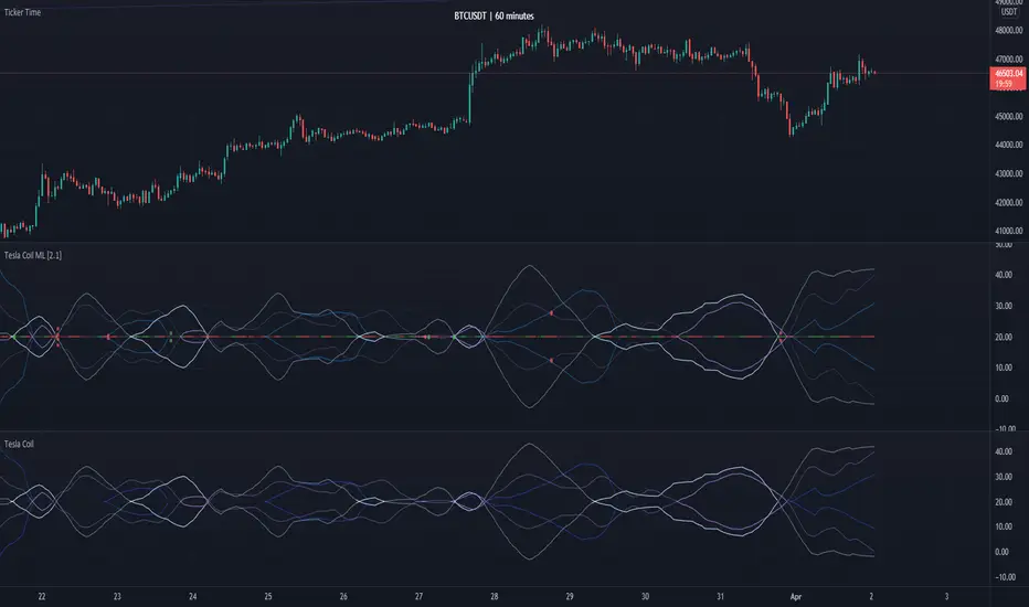
Tesla Coil MLThis is a re-implementation of @veryfid's wonderful Tesla Coil indicator to leverage basic Machine Learning Algorithms to help classify coil crossovers. The original Tesla Coil indicator requires extensive training and practice for the user to develop adequate intuition to interpret coil crossovers. The goal for this version is to help the user understand the underlying logic of the Tesla Coil indicator and provide a more intuitive way to interpret the indicator. The signals should be interpreted as suggestions rather than as a hard-coded set of rules.
NOTE: Please do NOT trade off the signals blindly. Always try to use your own intuition for understanding the coils and check for confluence with other indicators before initiating a trade.
Mean Shift Pivot ClusteringCore Concepts
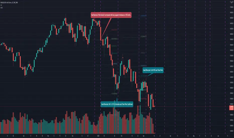
According to Jeff Greenblatt in his book "Breakthrough Strategies for Predicting Any Market", Fibonacci and Lucas sequences are observed repeated in the bar counts from local pivot highs/lows. They occur from high to high, low to high, high to low, or low to high. Essentially, this phenomenon is observed repeatedly from any pivot points on any time frame. Greenblatt combines this observation with Elliott Waves to predict the price and time reversals. However, I am no Elliottician so it was not easy for me to use this in a practical manner. I decided to only use the bar count projections and ignore the price. I projected a subset of Fibonacci and Lucas sequences along with the Fibonacci ratios from each pivot point. As expected, a projection from each pivot point resulted in a large set of plotted data and looks like a huge gong show of lines. Surprisingly, I did notice clusters and have observed those clusters to be fairly accurate.
Fibonacci Sequence: 1, 2, 3, 5, 8, 13, 21, 34...
Lucas Sequence: 2, 1, 3, 4, 7, 11, 18, 29, 47...
Fibonacci Ratios (converted to whole numbers): 23, 38, 50, 61, 78, 127, 161...
Light Bulb Moment
My eyes may suck at grouping the lines together but what about clustering algorithms? I chose to use a gimped version of Mean Shift because it doesn't require me to know in advance how many lines to expect like K-Means. Mean shift is computationally expensive and with Pinescript's 500ms timeout, I had to make due without the KDE. In other words, I skipped the weighting part but I may try to incorporate it in the future. The code is from Harrison Kinsley . He's a fantastic teacher!
Usage
Search Radius: how far apart should the bars be before they are excluded from the cluster? Try to stick with a figure between 1-5. Too large a figure will give meaningless results.
Pivot Offset: looks left and right X number of bars for a pivot. Same setting as the default TradingView pivot high/low script.
Show Lines Back: show historical predicted lines. (These can change)
Use this script in conjunction with Fibonacci price retracement/extension levels and/or other support/resistance levels. If it's no where near a support/resistance and there's a projected time pivot coming up, it's probably a fake out.
Notes
Re-painting is intended. When a new pivot is found, it will project out the Fib/Lucas sequences so the algorithm will run again with additional information.
The script is for informational and educational purposes only.
Do not use this indicator by itself to trade!
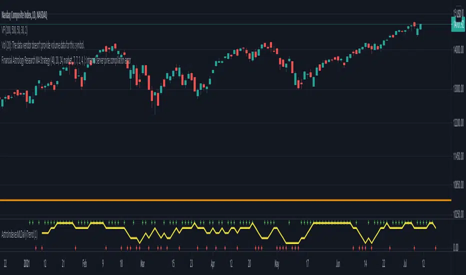
Financial Astrology Indexes ML Daily TrendDaily trend indicator based on financial astrology cycles detected with advanced machine learning techniques for some of the most important market indexes: DJI, UK100, SPX, IBC, IXIC, NI225, BANKNIFTY, NIFTY and GLD fund (not index) for Gold predictions. The daily price trend is forecasted through planets cycles (angular aspects, speed phases, declination zone), fast cycles are based on Moon, Mercury, Venus and Sun and Mid term cycles are based on Mars, Vesta and Ceres . The combination of all this cycles produce a daily price trend prediction that is encoded into a PineScript array using binary format "0 or 1" that represent sell and buy signals respectively. The indicator provides signals since 2021-01-01 to 2022-12-31, the past months signals purpose is to support backtesting of the indicator combined with other technical indicator entries like MAs, RSI or Stochastic . For future predictions besides 2022 a machine learning models re-train phase will be required.
When the signal moving average is increasing from 0 to 1 indicates an increase of buy force, when is decreasing from 1 to 0 indicates an increase in sell force, finally, when is sideways around the 0.4-0.6 area predicts a period of buy/sell forces equilibrium, traders indecision which result in a price congestion within a narrow price range.
We also have published same indicator for Crypto-Currencies research portfolio:
DISCLAIMER: This indicator is experimental and don’t provide financial or investment advice, the main purpose is to demonstrate the predictive power of financial astrology. Any allocation of funds following the documented machine learning model prediction is a high-risk endeavour and it’s the users responsibility to practice healthy risk management according to your situation.
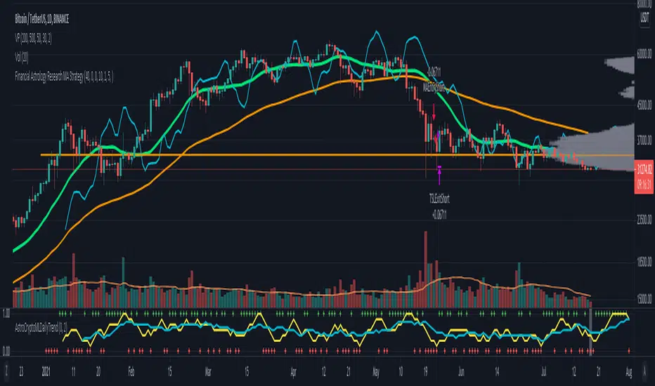
Financial Astrology Crypto ML Daily TrendThis daily trend indicator is based on financial astrology cycles detected with advanced machine learning techniques for the crypto-currencies research portfolio: ADA, BAT, BNB, BTC, DASH, EOS, ETC, ETH, LINK, LTC, XLM, XMR, XRP, ZEC and ZRX. The daily price trend is forecasted through this planets cycles (angular aspects, speed, declination), fast ones are based on Moon, Mercury, Venus and Sun and Mid term cycles are based on Mars, Vesta and Ceres. The combination of all this cycles produce a daily price trend prediction that is encoded into a PineScript array using binary format "0 or 1" that represent sell and buy signals respectively. The indicator provides signals since 2021-01-01 to 2022-12-31, the past months signals purpose is to support backtesting of the indicator combined with other technical indicator entries like MAs, RSI or Stochastic. For future predictions besides 2022 a machine learning models re-train phase will be required.
The resolution of this indicator is 1D, you can tune a parameter where you can determine how many future bars of daily trend are plotted and adjust an hours shift to anticipate future signals into current bar in order to produce a leading indicator effect to anticipate the trend changes with some hours of anticipation. Combined with technical analysis indicators this daily trend is very powerful because can help to produce approximately 60% of profitable signals based on the backtesting results. You can look at our open source Github repositories to validate accuracy using the backtesting strategies we have implemented in Jesse Crypto Trading Framework as proof of concept of the predictive potential of this indicator. Alternatively, we have implemented a PineScript strategy that use this indicator, just consider that we are pending to do signals update to the period July 2021 to December 2022: This strategy have accumulated more than 110 likes and many traders have validated the predictive power of Financial Astrology.
DISCLAIMER: This indicator is experimental and don’t provide financial or investment advice, the main purpose is to demonstrate the predictive power of financial astrology. Any allocation of funds following the documented machine learning model prediction is a high-risk endeavour and it’s the users responsibility to practice healthy risk management according to your situation.
Machine Learning: kNN-based Strategy (update)kNN-based Strategy (FX and Crypto)
Description:
This update to the popular kNN-based strategy features:
improvements in the business logic,
an adjustible k value for the kNN model,
one more feature (MOM),
a streamlined signal filter and
some other minor fixes.
Now this script works in all timeframes !
I intentionally decided to publish this script separately
in order for the users to see the differences.

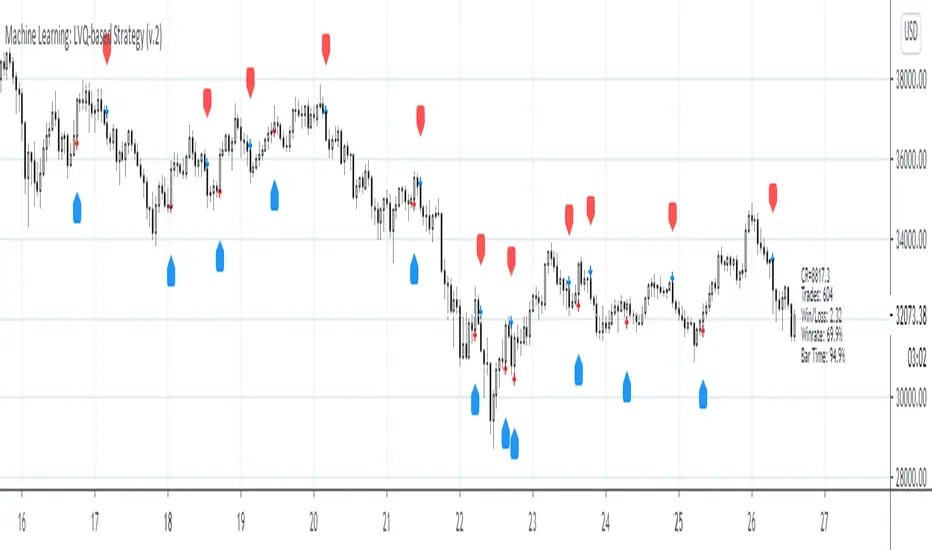
Machine Learning: LVQ-based StrategyLVQ-based Strategy (FX and Crypto)
Description:
Learning Vector Quantization (LVQ) can be understood as a special case of an artificial neural network, more precisely, it applies a winner-take-all learning-based approach. It is based on prototype supervised learning classification task and trains its weights through a competitive learning algorithm.
Algorithm:
Initialize weights
Train for 1 to N number of epochs
- Select a training example
- Compute the winning vector
- Update the winning vector
Classify test sample
The LVQ algorithm offers a framework to test various indicators easily to see if they have got any *predictive value*. One can easily add cog, wpr and others.
Note: TradingViews's playback feature helps to see this strategy in action. The algo is tested with BTCUSD/1Hour.
Warning: This is a preliminary version! Signals ARE repainting.
***Warning***: Signals LARGELY depend on hyperparams (lrate and epochs).
Style tags: Trend Following, Trend Analysis
Asset class: Equities, Futures, ETFs, Currencies and Commodities
Dataset: FX Minutes/Hours+++/Days
Machine Learning: Logistic RegressionMulti-timeframe Strategy based on Logistic Regression algorithm
Description:
This strategy uses a classic machine learning algorithm that came from statistics - Logistic Regression (LR).
The first and most important thing about logistic regression is that it is not a 'Regression' but a 'Classification' algorithm. The name itself is somewhat misleading. Regression gives a continuous numeric output but most of the time we need the output in classes (i.e. categorical, discrete). For example, we want to classify emails into “spam” or 'not spam', classify treatment into “success” or 'failure', classify statement into “right” or 'wrong', classify election data into 'fraudulent vote' or 'non-fraudulent vote', classify market move into 'long' or 'short' and so on. These are the examples of logistic regression having a binary output (also called dichotomous).
You can also think of logistic regression as a special case of linear regression when the outcome variable is categorical, where we are using log of odds as dependent variable. In simple words, it predicts the probability of occurrence of an event by fitting data to a logit function.
Basically, the theory behind Logistic Regression is very similar to the one from Linear Regression, where we seek to draw a best-fitting line over data points, but in Logistic Regression, we don’t directly fit a straight line to our data like in linear regression. Instead, we fit a S shaped curve, called Sigmoid, to our observations, that best SEPARATES data points. Technically speaking, the main goal of building the model is to find the parameters (weights) using gradient descent.
In this script the LR algorithm is retrained on each new bar trying to classify it into one of the two categories. This is done via the logistic_regression function by updating the weights w in the loop that continues for iterations number of times. In the end the weights are passed through the sigmoid function, yielding a prediction.
Mind that some assets require to modify the script's input parameters. For instance, when used with BTCUSD and USDJPY, the 'Normalization Lookback' parameter should be set down to 4 (2,...,5..), and optionally the 'Use Price Data for Signal Generation?' parameter should be checked. The defaults were tested with EURUSD.
Note: TradingViews's playback feature helps to see this strategy in action.
Warning: Signals ARE repainting.
Style tags: Trend Following, Trend Analysis
Asset class: Equities, Futures, ETFs, Currencies and Commodities
Dataset: FX Minutes/Hours/Days

Machine Learning: Perceptron-based strategyPerceptron-based strategy
Description:
The Learning Perceptron is the simplest possible artificial neural network (ANN), consisting of just a single neuron and capable of learning a certain class of binary classification problems. The idea behind ANNs is that by selecting good values for the weight parameters (and the bias), the ANN can model the relationships between the inputs and some target.
Generally, ANN neurons receive a number of inputs, weight each of those inputs, sum the weights, and then transform that sum using a special function called an activation function. The output of that activation function is then either used as the prediction (in a single neuron model) or is combined with the outputs of other neurons for further use in more complex models.
The purpose of the activation function is to take the input signal (that’s the weighted sum of the inputs and the bias) and turn it into an output signal. Think of this activation function as firing (activating) the neuron when it returns 1, and doing nothing when it returns 0. This sort of computation is accomplished with a function called step function: f(z) = {1 if z > 0 else 0}. This function then transforms any weighted sum of the inputs and converts it into a binary output (either 1 or 0). The trick to making this useful is finding (learning) a set of weights that lead to good predictions using this activation function.
Training our perceptron is simply a matter of initializing the weights to zero (or random value) and then implementing the perceptron learning rule, which just updates the weights based on the error of each observation with the current weights. This has the effect of moving the classifier’s decision boundary in the direction that would have helped it classify the last observation correctly. This is achieved via a for loop which iterates over each observation, making a prediction of each observation, calculating the error of that prediction and then updating the weights accordingly. In this way, weights are gradually updated until they converge. Each sweep through the training data is called an epoch.
In this script the perceptron is retrained on each new bar trying to classify this bar by drawing the moving average curve above or below the bar.
This script was tested with BTCUSD, USDJPY, and EURUSD.
Note: TradingViews's playback feature helps to see this strategy in action.
Warning: Signals ARE repainting.
Style tags: Trend Following, Trend Analysis
Asset class: Equities, Futures, ETFs, Currencies and Commodities
Dataset: FX Minutes/Hours+/Days
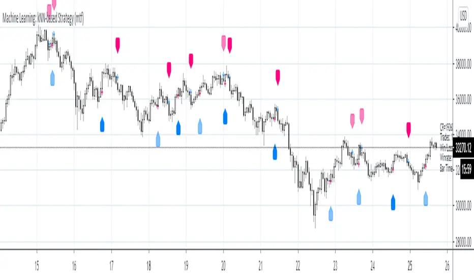
Machine Learning: kNN-based Strategy (mtf)This is a multi-timeframe version of the kNN-based strategy.
Machine Learning: kNN-based StrategykNN-based Strategy (FX and Crypto)
Description:
This strategy uses a classic machine learning algorithm - k Nearest Neighbours (kNN) - to let you find a prediction for the next (tomorrow's, next month's, etc.) market move. Being an unsupervised machine learning algorithm, kNN is one of the most simple learning algorithms.
To do a prediction of the next market move, the kNN algorithm uses the historic data, collected in 3 arrays - feature1, feature2 and directions, - and finds the k-nearest
neighbours of the current indicator(s) values.
The two dimensional kNN algorithm just has a look on what has happened in the past when the two indicators had a similar level. It then looks at the k nearest neighbours,
sees their state and thus classifies the current point.
The kNN algorithm offers a framework to test all kinds of indicators easily to see if they have got any *predictive value*. One can easily add cog, wpr and others.
Note: TradingViews's playback feature helps to see this strategy in action.
Warning: Signals ARE repainting.
Style tags: Trend Following, Trend Analysis
Asset class: Equities, Futures, ETFs, Currencies and Commodities
Dataset: FX Minutes/Hours+++/Days
Machine Learning / Longs [Experimental]Hello Traders/Programmers,
For long time I thought that if it's possible to make a script that has own memory and criterias in Pine. it would learn and find patterns as images according to given criterias. after we have arrays of strings, lines, labels I tried and made this experimental script. The script works only for Long positions.
Now lets look at how it works:
On each candle it creates an image of last 8 candles. before the image is created it finds highest/lowest levels of 8 candles, and creates a string with the lengths 64 (8 * 8). and for each square, it checks if it contains wick, green or red body, green or red body with wicks. see the following picture:
Each square gets the value:
0: nothing in it
1: only wick in it
2: only red body in it
3. only green body in it
4: red body and wick in it
5: green body and wick in it
And then it checks if price went up equal or higher than user-defined profit. if yes then it adds the image to the memory/array. and I call this part as Learning Part.
what I mean by image is:
if there is 1 or more element in the memory, it creates image for current 8 candles and checks the memory if there is a similar images. If the image has similarity higher than user-defined similarty level then if show the label "Matched" and similarity rate and the image in the memory. if it find any with the similarity rate is equal/greater than user-defined level then it stop searching more.
As an example matched image:
and then price increased and you got the profit :)
Options:
Period: if there is possible profit higher than user-defined minimum profit in that period, it checks the images from 2. to X. bars.
Min Profit: you need to set the minimum expected profit accordingly. for example in 1m chart don't enter %10 as min profit :)
Similarity Rate: as told above, you can set minimum similarity rate, higher similarity rate means better results but if you set higher rates, number of images will decrease. set it wisely :)
Max Memory Size: you can set number of images (that gives the profit equal/higher than you set) to be saved that in memory
Change Bar Color: optionally it can change bar colors if current image is found in the memory
Current version of the script doesn't check if the price reach the minimum profit target, so no statistics.
This is completely experimental work and I made it for fun. No one or no script can predict the future. and you should not try to predict the future.
P.S. it starts searching on last bar, it doesn't check historical bars. if you want you should check it in replay mode :)
if you get calculation time out error then hide/unhide the script. ;)
Enjoy!

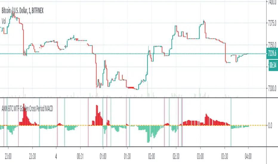
ANN BTC MTF Golden Cross Period MACDHi, this is the MACD version of the ANN BTC Multi Timeframe Script.
The MACD Periods were approximated to the Golden Cross values.
MACD Lengths :
Signal Length = 25
Fast Length = 50
Slow Length = 200
Regards.
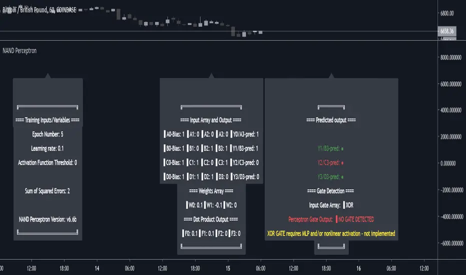
NAND PerceptronExperimental NAND Perceptron based upon Python template that aims to predict NAND Gate Outputs. A Perceptron is one of the foundational building blocks of nearly all advanced Neural Network layers and models for Algo trading and Machine Learning.
The goal behind this script was threefold:
To prove and demonstrate that an ACTUAL working neural net can be implemented in Pine, even if incomplete.
To pave the way for other traders and coders to iterate on this script and push the boundaries of Tradingview strategies and indicators.
To see if a self-contained neural network component for parameter optimization within Pinescript was hypothetically possible.
NOTE: This is a highly experimental proof of concept - this is NOT a ready-made template to include or integrate into existing strategies and indicators, yet (emphasis YET - neural networks have a lot of potential utility and potential when utilized and implemented properly).
Hardcoded NAND Gate outputs with Bias column (X0):
// NAND Gate + X0 Bias and Y-true
// X0 // X1 // X2 // Y
// 1 // 0 // 0 // 1
// 1 // 0 // 1 // 1
// 1 // 1 // 0 // 1
// 1 // 1 // 1 // 0
Column X0 is bias feature/input
Column X1 and X2 are the NAND Gate
Column Y is the y-true values for the NAND gate
yhat is the prediction at that timestep
F0,F1,F2,F3 are the Dot products of the Weights (W0,W1,W2) and the input features (X0,X1,X2)
Learning rate and activation function threshold are enabled by default as input parameters
Uncomment sections for more training iterations/epochs:
Loop optimizations would be amazing to have for a selectable length for training iterations/epochs but I'm not sure if it's possible in Pine with how this script is structured.
Error metrics and loss have not been implemented due to difficulty with script length and iterations vs epochs - I haven't been able to configure the input parameters to successfully predict the right values for all four y-true values for the NAND gate (only been able to get 3/4; If you're able to get all four predictions to be correct, let me know, please).
// //---- REFERENCE for final output
// A3 := 1, y0 true
// B3 := 1, y1 true
// C3 := 1, y2 true
// D3 := 0, y3 true
PLEASE READ: Source article/template and main code reference:
towardsdatascience.com
towardsdatascience.com
towardsdatascience.com
CBOE PCR Factor Dependent Variable Odd Generator This script is the my Dependent Variable Odd Generator script :
with the Put / Call Ratio ( PCR ) appended, only for CBOE and the instruments connected to it.
For CBOE this script is more accurate and faster than Dependent Variable Odd Generator. And the stagnant market odds are better and more realistic.
Do not use for timeframe periods less than 1 day.
Because PCR data may give repaint error.
My advice is to use the 1-week bars to gain insight into your analysis.
This code is open source under the MIT license. If you have any improvements or corrections to suggest, please send me a pull request via the github repository github.com
I hope it will help your work.Best regards!

ANN MACD (BTC)
Logic is correct.
But I prefer to say experimental because the sample set is narrow. (300 columns)
Let's start:
6 inputs : Volume Change , Bollinger Low Band chg. , Bollinger Mid Band chg., Bollinger Up Band chg. , RSI change , MACD histogram change.
1 output : Future bar change (Historical)
Training timeframe : 15 mins (Analysis TF > 4 hours (My opinion))
Learning cycles : 337
Training error: 0.009999
Input columns: 6
Output columns: 1
Excluded columns: 0
Grid
Training example rows: 301
Validating example rows: 0
Querying example rows: 0
Excluded example rows: 0
Duplicated example rows: 0
Network
Input nodes connected: 6
Hidden layer 1 nodes: 8
Hidden layer 2 nodes: 0
Hidden layer 3 nodes: 0
Output nodes: 1
Learning rate : 0.6 Momentum : 0.8
More info :
EDIT : This code is open source under the MIT License. If you have any improvements or corrections to suggest, please send me a pull request via the github repository github.com