ASFX - Automatic VWAPs & Key LevelsAutomate your AVWAPs and key levels for day trading! NY Market open VWAP, Previous day NY VWAP, and more are included. Inital Balance and Opening Range are also automated.
ความผันผวน

Value Charts by Mark Helweg1. Introduction
This script is a simplified implementation of the Value Charts concept introduced by Mark Helweg and David Stendahl in their work on “Dynamic Trading Indicators”. It converts raw price into value units by normalizing distance from a dynamic fair‑value line, making it easier to see when price is relatively overvalued or undervalued across different markets and timeframes. The code focuses on plotting Value Chart candlesticks and clean visual bands, keeping the logic close to the original idea while remaining lightweight for intraday and swing trading.
2. Key Features
- Dynamic fair‑value axis
Uses a moving average of the chosen price source as the fair‑value line and a volatility‑based deviation (smoothed True Range) to scale all price moves into comparable value units.
- Normalized Value Chart candlesticks
OHLC prices are transformed into value units and displayed as a dedicated candlestick panel, visually similar to standard candles but detached from raw price, highlighting relative extremes instead of absolute levels.
- Custom upper and lower visual limits
User‑defined upper and lower bands frame the majority of action and emphasize extreme value zones, helping the trader spot potential exhaustion or mean‑reversion conditions at a glance.
- Clean, publishing‑friendly layout
Only the normalized candles and three simple reference lines (top, bottom, zero) are plotted, keeping the chart uncluttered and compliant with presentation standards for published scripts.
3. How to Use
1. Attach the indicator to a separate pane (overlay = false) on any market and timeframe you trade.
2. Set the “Period (Value Chart)” to control how fast the fair‑value line adapts: shorter values react more quickly, longer values smooth more.
3. Adjust the “Volatility Factor” so that most candles stay between the upper and lower limits, with only true extremes touching or exceeding them.
4. Use the Value Chart candlesticks as a relative overbought/oversold tool:
- Candles pressing into the Top band suggest overvalued conditions and potential for pullbacks or reversions.
- Candles pressing into the Bottom band suggest undervalued conditions and potential for bounces.
5. Combine the signals with your existing price‑action, volume, or trend‑filter rules on the main chart; the Value Chart panel is designed as a context and timing tool, not a standalone trading system.

Combined: Net Volume, RSI & ATR# Combined: Net Volume, RSI & ATR Indicator
## Overview
This custom TradingView indicator overlays **Net Volume** and **RSI (Relative Strength Index)** on the same chart panel, with RSI scaled to match the visual range of volume spikes. It also displays **ATR (Average True Range)** values in a table.
## Key Features
### Net Volume
- Calculates buying vs selling pressure by analyzing lower timeframe data
- Displays as a **yellow line** centered around zero
- Automatically selects optimal timeframe or allows manual override
- Shows net buying pressure (positive values) and selling pressure (negative values)
### RSI (Relative Strength Index)
- Traditional 14-period RSI displayed as a **blue line**
- **Overlays directly on the volume chart** - scaled to match volume spike heights
- Includes **70/30 overbought/oversold levels** (shown as dotted red/green lines)
- Adjustable scale factor to fine-tune visual sizing relative to volume
- Optional **smoothing** with multiple moving average types (SMA, EMA, RMA, WMA, VWMA)
- Optional **Bollinger Bands** around RSI smoothing line
- **Divergence detection** - identifies regular bullish/bearish divergences with labels
### ATR (Average True Range)
- Displays current ATR value in a **table at top-right corner**
- Configurable period length (default: 50)
- Multiple smoothing methods: RMA, SMA, EMA, or WMA
- Helps assess current market volatility
## Use Cases
- **Momentum & Volume Confirmation**: See if RSI trends align with net volume flows
- **Divergence Trading**: Automatically spots when price makes new highs/lows but RSI doesn't
- **Volatility Assessment**: Monitor ATR for position sizing and stop-loss placement
- **Overbought/Oversold + Volume**: Identify exhaustion when RSI hits extremes with volume spikes
## Customization
All components can be toggled on/off independently. RSI scale factor allows you to adjust how prominent the RSI line appears relative to volume bars.

BTC Dynamic Volatility Trend Backtested from 2017 to present, this strategy has delivered a staggering 7100%+ cumulative return. It doesn't just track the market; it dominates it. By capturing major trends and strictly limiting drawdowns, it has significantly outperformed the standard 'Buy & Hold' BTC strategy, proving its ability to generate massive alpha across multiple bull and bear cycles.
自 2017 年至今,本策略实现了惊人的 7100%+ 累计收益率。它不仅仅是跟随市场,更是超越了市场。通过精准捕捉主升浪并严格控制回撤,该策略在穿越多轮牛熊周期后,大幅度跑赢了比特币‘买入持有’(Buy & Hold)的基准收益,展现了极致的阿尔法(Alpha)捕捉能力。"
Introduction :Simplicity is the ultimate sophistication. This strategy is designed specifically for Bitcoin (BTC), capturing its unique characteristics: high volatility, frequent fakeouts, and massive trend persistence. It abandons complex indicators in favor of a robust logic: "Follow the Trend, Filter the Noise, Let Profits Run."
Core Logic
Trend Filter (Fibonacci EMA 144): We use the 144-period Exponential Moving Average as the baseline. Longs are only taken above this line, and shorts only below. This keeps you on the right side of the major trend.
Volatility Breakout (Donchian Channel 20): Entries are triggered only when price breaks the 20-day high (for longs) or low (for shorts). This confirms momentum and avoids trading in chop.
Dynamic Risk Management (ATR Chandelier Exit):
Instead of fixed % stops, we use Average True Range (ATR) to calculate stop losses.
The Ratchet Mechanism: The stop loss moves up with the price but never moves down (for longs). This locks in profits automatically as the trend develops and exits immediately when volatility turns against you.
Why Use This Strategy?
Zero Repainting: All signals are confirmed.
No Curve Fitting: Uses classic parameters (144, 20) that have worked for decades.
Mental Peace: The strategy handles the exit. You don't need to guess where to sell. It holds through minor corrections and exits only when the trend truly reverses.
Settings
Leverage %: Adjust your position size based on equity (default 100% = 1x).
Timeframe: Recommended for 4H charts.
中文版 (Chinese Version)
简介 :大道至简。本策略专为 比特币 (BTC) 设计,针对其高波动、假突破多但趋势爆发力强的特点,摒弃了复杂的过度拟合指标,回归交易本质:“顺大势,滤噪音,截断亏损,让利润奔跑”。
核心逻辑
趋势过滤器 (斐波那契 EMA 144): 使用 144 周期指数移动平均线作为多空分水岭。价格在均线之上只做多,之下只做空。这能有效过滤掉大部分震荡市的噪音。
波动率突破 (唐奇安通道 20): 只有当价格突破过去 20 根 K 线的最高价(做多)或最低价(做空)时才进场。这确保了我们只在趋势确立的瞬间入场。
动态风控 (ATR 吊灯止损):
拒绝固定点数止损,使用 ATR(平均真实波幅)根据市场热度动态计算安全距离。
棘轮机制: 止损线会跟随价格上涨而上移,但绝不会下移(做多时)。这实现了自动化的“利润锁定”,既能扛住正常的波动回调,又能在大势反转时果断离场。
策略优势
绝不重绘: 所有信号均为收盘确认或实时触价。
拒绝拟合: 使用经过数十年市场验证的经典参数组合。
心态管理: 策略全自动管理出场。你不需要纠结何时止盈,它会帮你吃到完整的鱼身,直到趋势结束。
使用建议
资金管理: 可通过参数调整仓位占比(默认 100% = 1倍杠杆)。
推荐周期: 建议在4小时 图表上运行效果最佳。
US Market Long Horizon Momentum Summary in one paragraph
US Market Long Horizon Momentum is a trend following strategy for US index ETFs and futures built around a single eighteen month time series momentum measure. It helps you stay long during persistent bull regimes and step aside or flip short when long term momentum turns negative.
Scope and intent
• Markets. Large cap US equity indices, liquid US index ETFs, index futures
• Timeframes. 4h/ Daily charts
• Default demo used in the publication. SPY on 4h timeframe chart
• Purpose. Provide a minimal long bias index timing model that can reduce deep drawdowns and capture major cycles without parameter mining
• Limits. This is a strategy. Orders are simulated on standard candles only
Originality and usefulness
• Unique concept or fusion. One unscaled multiple month log return of an external benchmark symbol drives all entries and exits, with optional volatility targeting as a single risk control switch.
• Failure mode addressed. Fully passive buy and hold ignores the sign of long horizon momentum and can sit through multi year drawdowns. This script offers a way to step down risk in prolonged negative momentum without chasing short term noise.
• Testability. All parameters are visible in Inputs and the momentum series is plotted so users can verify every regime change in the Tester and on price history.
• Portable yardstick. The log return over a fixed window is a unit that can be applied to any liquid symbol with daily data.
Method overview in plain language
The method looks at how far the benchmark symbol has moved in log return terms over an eighteen month window in our example. If that long horizon return is positive the strategy allows a long stance on the traded symbol. If it is negative and shorts are enabled the strategy can flip short, otherwise it goes flat. There is an optional realised volatility estimate on the traded symbol that can scale position size toward a target annual volatility, but in the default configuration the model uses unit leverage and only the sign of momentum matters.
Base measures
Return basis. The core yardstick is the natural log of close divided by the close eighteen months ago on the benchmark symbol. Daily log returns of the traded symbol feed the realised volatility estimate when volatility targeting is enabled.
Components
• Component one Momentum eighteen months. Log of benchmark close divided by its close mom_lookback bars ago. Its sign defines the trend regime. No extra smoothing is applied beyond the long window itself.
• Component two Realised volatility optional. Standard deviation of daily log returns on the traded symbol over sixty three days. Annualised by the square root of 252. Used only when volatility targeting is enabled.
• Optional component Volatility targeting. Converts target annual volatility and realised volatility into a leverage factor clipped by a maximum leverage setting.
Fusion rule
The model uses a simple gate. First compute the sign of eighteen month log momentum on the benchmark symbol. Optionally compute leverage from volatility. The sign decides whether the strategy wants to be long, short, or flat. Leverage only rescales position size when enabled and does not change direction.
Signal rule
• Long suggestion. When eighteen month log momentum on the benchmark symbol is greater than zero, the strategy wants to be long.
• Short suggestion. When that log momentum is less than zero and shorts are allowed, the strategy wants to be short. If shorts are disabled it stays flat instead.
• Wait state. When the log momentum is exactly zero or history is not long enough the strategy stays flat.
• In position. In practice the strategy sits IN LONG while the sign stays positive and flips to IN SHORT or flat only when the sign changes.
Inputs with guidance
Setup
• Momentum Lookback (months). Controls the horizon of the log return on the benchmark symbol. Typical range 6 to 24 months. Raising it makes the model slower and more selective. Lowering it makes it more reactive and sensitive to medium term noise.
• Symbol. External symbol used for the momentum calculation, SPY by default. Changing it lets you time other indices or run signals from a benchmark while trading a correlated instrument.
Logic
• Allow Shorts. When true the strategy will open short positions during negative momentum regimes. When false it will stay flat whenever momentum is negative. Practical setting is tied to whether you use a margin account or an ETF that supports shorting.
Internal risk parameters (not exposed as inputs in this version) are:
• Target Vol (annual). Target annual volatility for volatility targeting, default 0.2.
• Vol Lookback (days). Window for realised volatility, default 63 trading days.
• Max Leverage. Cap on leverage when volatility targeting is enabled, default 2.
Usage recipes
Swing continuation
• Signal timeframe. Use the daily chart.
• Benchmark symbol. Leave at SPY for US equity index exposure.
• Momentum lookback. Eighteen months as a default, with twelve months as an alternative preset for a faster swing bias.
Properties visible in this publication
• Initial capital. 100000
• Base currency. USD
• Default order size method. 5% of the total capital in this example
• Pyramiding. 0
• Commission. 0.03 percent
• Slippage. 3 ticks
• Process orders on close. On
• Bar magnifier. Off
• Recalculate after order is filled. Off
• Calc on every tick. Off
• All request.security calls use lookahead = barmerge.lookahead_off
Realism and responsible publication
The strategy is for education and research only. It does not claim any guaranteed edge or future performance. All results in Strategy Tester are hypothetical and depend on the data vendor, costs, and slippage assumptions. Intrabar motion is not modeled inside daily bars so extreme moves and gaps can lead to fills that differ from live trading. The logic is built for standard candles and should not be used on synthetic chart types for execution decisions.
Performance is sensitive to regime structure in the US equity market, which may change over time. The strategy does not protect against single day crash risk inside bars and does not model gap risk explicitly. Past behavior of SPY and the momentum effect does not guarantee future persistence.
Honest limitations and failure modes
• Long sideways regimes with small net change over eighteen months can lead to whipsaw around the zero line.
• Very sharp V shaped reversals after deep declines will often be missed because the model waits for momentum to turn positive again.
• The sample size in a full SPY history is small because regime changes are infrequent, so any test must be interpreted as indicative rather than statistically precise.
• The model is highly dependent on the chosen lookback. Users should test nearby values and validate that behavior is qualitatively stable.
Legal
Education and research only. Not investment advice. You are responsible for your own decisions. Always test on historical data and in simulation with realistic costs before any live use.

RiskCraft - Advanced Risk Management SystemRiskCraft – Risk Intelligence Dashboard
Trade like you actually respect risk
"I know the setup looks good… but how much am I actually risking right now?"
RiskCraft is an open-source Pine Script v6 indicator that keeps risk transparent directly on the chart. It is not a signal generator; it is a risk desk that calculates size, frames volatility, and reminds you when your behaviour drifts away from the plan.
Core utilities
Calculates professional-style position sizing in real time.
Reads volatility and market regime before position size is confirmed.
Adjusts risk based on the trader’s emotional state and confidence inputs.
Maps session risk across Asian, London, and New York hours.
Draws exactly one stop line and one target line in the preferred direction.
Provides rotating education tips plus contextual warnings when risk escalates.
It is intentionally conservative and keeps you in the game long enough for any separate entry logic to matter.
---
Chart layout checklist
Use a clean chart on a liquid symbol (e.g., AMEX:SPY or major FX pairs).
Main RiskCraft dashboard placed on the right edge.
Session Risk box on the left with UTC time visible.
Floating risk badge above price.
Stop/target guide lines enabled.
Education panel visible in the bottom-right corner.
---
1. On-chart components
Right-side dashboard : account risk %, position size/value, stop, target, risk/reward, regime, trend strength, emotional state, behavioural score, correlation, and preferred trade direction.
Session Risk box : highlights active session (Asian, London, NY), current UTC time, and risk label (High/Med/Low) per session.
Floating risk badge : keeps actual account risk percent visible with colour-coded wording from Ultra Cautious to Very Aggressive.
Stop/target lines : exactly one dashed stop and one dashed target aligned with the preferred bias.
Education panel : rotates core principles and AI-style warnings tied to volatility, risk %, and behaviour flags.
---
2. Volatility engine – ATR with context 📈
atr = ta.atr(atrLength)
atrPercent = (atr / close) * 100
atrSMA = ta.sma(atr, atrLength)
volatilityRatio = atr / atrSMA
isHighVol = volatilityRatio > volThreshold
ATR vs ATR SMA shows how wild price is relative to recent history.
Volatility ratio above the threshold flips isHighVol , which immediately trims risk.
An ATR percentile rank over the last 100 bars indicates calm versus chaotic regimes.
Daily ATR sampling via request.security() gives higher time-frame context for intraday sessions.
When volatility spikes the script dials position size down automatically instead of cheering for maximum exposure.
---
3. Market regime radar – Danger or Drift 🌊
ema20 = ta.ema(close, 20)
ema50 = ta.ema(close, 50)
ema200 = ta.ema(close, 200)
trendScore = (close > ema20 ? 1 : -1) +
(ema20 > ema50 ? 1 : -1) +
(ema50 > ema200 ? 1 : -1)
= ta.dmi(14, 14)
Regimes covered:
Danger : high volatility with weak trend.
Volatile : volatility elevated but structure still directional.
Choppy : low ADX and noisy action.
Trending : directional flows without extreme volatility.
Mixed : anything between.
Each regime maps to a 1–10 risk score and a multiplier that feeds the final position size. Danger and Choppy clamp size; Trending restores normal risk.
---
4. Behaviour engine – trader inputs matter 🧠
You provide:
Emotional state : Confident, Neutral, FOMO, Revenge, Fearful.
Confidence : slider from 1 to 10.
Toggle for behavioural adjustment on/off.
Behind the scenes:
Each state triggers an emotional multiplier .
Confidence produces a confidence multiplier .
Combined they form behavioralFactor and a 0–100 Behavioural Score .
High-risk emotions or low conviction clamp the final risk. Calm inputs allow normal size. The dashboard prints both fields to keep accountability on-screen.
---
5. Correlation guardrail – avoid stacking identical risk 📊
Optional correlation mode compares the active symbol to a reference (default AMEX:SPY ):
corrClose = request.security(correlationSymbol, timeframe.period, close)
priceReturn = ta.change(close) / close
corrReturn = ta.change(corrClose) / corrClose
correlation = calcCorrelation()
Absolute correlation above the threshold applies a correlation multiplier (< 1) to reduce size.
Dashboard row shows the live correlation and reference ticker.
When disabled, the row simply echoes the current symbol, keeping the table readable.
---
6. Position sizing engine – heart of the script 💰
baseRiskAmount = accountSize * (baseRiskPercent / 100)
adjustedRisk = baseRiskAmount * behavioralFactor *
regimeAdjustment * volAdjustment *
correlationAdjustment
finalRiskAmount = math.min(adjustedRisk,
accountSize * (maxRiskCap / 100))
stopDistance = atr * atrStopMultiplier
takeProfit = atr * atrTargetMultiplier
positionSize = stopDistance > 0 ? finalRiskAmount / stopDistance : 0
positionValue = positionSize * close
Outputs shown on the dashboard:
Position size in units and value in currency.
Actual risk % back on account after adjustments.
Risk/Reward derived from ATR-based stop and target.
---
7. Intelligent trade direction – bias without signals 🎯
Direction score ingredients:
EMA stack alignment.
Price versus EMA20.
RSI momentum relative to 50.
MACD line vs signal.
Directional Movement (DI+/DI–).
The resulting Trade Direction row prints LONG, SHORT, or NEUTRAL. No orders are generated—this is guidance so you only risk capital when the structure supports it.
---
8. Stop/target guide lines – two lines only ✂️
if showStopLines
if preferLong
// long stop below, target above
else if preferShort
// short stop above, target below
Lines refresh each bar to keep clutter low.
When the direction score is neutral, no lines appear.
Use them as visual anchors, not auto-orders.
---
9. Session Risk map – global volatility clock 🌍
Tracks Asian, London, and New York windows via UTC.
Computes average ATR per session versus global ATR SMA.
Labels each session High/Med/Low and colours the cells accordingly.
Top row shows the active session plus current UTC time so you always know the regime you are trading.
One glance tells you whether you are trading quiet drift or the part of the day that hunts stops.
---
10. Floating risk badge – honesty above price 🪪
Text ranges from Ultra Cautious through Very Aggressive.
Colour matches the risk palette inputs (High/Med/Low).
Updates on the last bar only, keeping historical clutter off the chart.
Account risk becomes impossible to ignore while you stare at price.
---
11. Education engine & warnings 📚
Rotates evergreen principles (risk 1–2%, journal trades, respect plan).
Triggers contextual warnings when volatility and risk % conflict.
Flags when emotional state = FOMO or Revenge.
Highlights sub-standard risk/reward setups.
When multiple danger flags stack, an AI-style warning overrides the tip text so you can course-correct before capital is exposed.
---
12. Alerts – hard guard rails 🚨
Excessive Risk Alert : actual risk % crosses custom threshold.
High Volatility Alert : ATR behaviour signals danger regime.
Emotional State Warning : FOMO or Revenge selected.
Poor Risk/Reward Alert : risk/reward drops below your standard.
All alerts reinforce discipline; none suggest entries or exits.
---
13. Multi-market behaviour 🕒
Intraday (1m–1h): session box and badge react quickly; ideal for scalpers needing constant risk context.
Higher time frames (1D–1W): dashboard shifts slowly, supporting swing planning.
Asset classes confirmed in validation: crypto majors, large-cap equities, indices, major FX pairs, and liquid commodities.
Risk logic is price-based, so it adapts across markets without bespoke tuning.
15. Key inputs & recommended defaults
Account Size : 10,000 (modify to match actual account; min 100).
Base Risk % : 1.0 with a Maximum Risk Cap of 2.5%.
ATR Period : 14, Stop Multiplier 2.0, Target Multiplier 3.0.
High Vol Threshold : 1.5 for ATR ratio.
Behavioural Adjustment : enabled by default; disable for fixed risk.
Correlation Check : optional; default symbol AMEX:SPY , threshold 0.7.
Display toggles : main dashboard, risk badge, session map, education panel, and stop lines can be individually disabled to reduce clutter.
16. Usage notes & limits
Indicator mode only; no automated entries or exits.
Trade history panel intentionally disabled (requires strategy context).
Correlation analysis depends on additional data requests and may lag slightly on illiquid symbols.
Session timing uses UTC; adjust expectations if you trade localized instruments.
HTF ATR sampling uses daily data, so bar replay on lower charts may show brief data gaps while HTF loads.
What does everyone think RISK really means?

Volatility Risk PremiumTHE INSURANCE PREMIUM OF THE STOCK MARKET
Every day, millions of investors face a fundamental question that has puzzled economists for decades: how much should protection against market crashes cost? The answer lies in a phenomenon called the Volatility Risk Premium, and understanding it may fundamentally change how you interpret market conditions.
Think of the stock market like a neighborhood where homeowners buy insurance against fire. The insurance company charges premiums based on their estimates of fire risk. But here is the interesting part: insurance companies systematically charge more than the actual expected losses. This difference between what people pay and what actually happens is the insurance premium. The same principle operates in financial markets, but instead of fire insurance, investors buy protection against market volatility through options contracts.
The Volatility Risk Premium, or VRP, measures exactly this difference. It represents the gap between what the market expects volatility to be (implied volatility, as reflected in options prices) and what volatility actually turns out to be (realized volatility, calculated from actual price movements). This indicator quantifies that gap and transforms it into actionable intelligence.
THE FOUNDATION
The academic study of volatility risk premiums began gaining serious traction in the early 2000s, though the phenomenon itself had been observed by practitioners for much longer. Three research papers form the backbone of this indicator's methodology.
Peter Carr and Liuren Wu published their seminal work "Variance Risk Premiums" in the Review of Financial Studies in 2009. Their research established that variance risk premiums exist across virtually all asset classes and persist over time. They documented that on average, implied volatility exceeds realized volatility by approximately three to four percentage points annualized. This is not a small number. It means that sellers of volatility insurance have historically collected a substantial premium for bearing this risk.
Tim Bollerslev, George Tauchen, and Hao Zhou extended this research in their 2009 paper "Expected Stock Returns and Variance Risk Premia," also published in the Review of Financial Studies. Their critical contribution was demonstrating that the VRP is a statistically significant predictor of future equity returns. When the VRP is high, meaning investors are paying substantial premiums for protection, future stock returns tend to be positive. When the VRP collapses or turns negative, it often signals that realized volatility has spiked above expectations, typically during market stress periods.
Gurdip Bakshi and Nikunj Kapadia provided additional theoretical grounding in their 2003 paper "Delta-Hedged Gains and the Negative Market Volatility Risk Premium." They demonstrated through careful empirical analysis why volatility sellers are compensated: the risk is not diversifiable and tends to materialize precisely when investors can least afford losses.
HOW THE INDICATOR CALCULATES VOLATILITY
The calculation begins with two separate measurements that must be compared: implied volatility and realized volatility.
For implied volatility, the indicator uses the CBOE Volatility Index, commonly known as the VIX. The VIX represents the market's expectation of 30-day forward volatility on the S&P 500, calculated from a weighted average of out-of-the-money put and call options. It is often called the "fear gauge" because it rises when investors rush to buy protective options.
Realized volatility requires more careful consideration. The indicator offers three distinct calculation methods, each with specific advantages rooted in academic literature.
The Close-to-Close method is the most straightforward approach. It calculates the standard deviation of logarithmic daily returns over a specified lookback period, then annualizes this figure by multiplying by the square root of 252, the approximate number of trading days in a year. This method is intuitive and widely used, but it only captures information from closing prices and ignores intraday price movements.
The Parkinson estimator, developed by Michael Parkinson in 1980, improves efficiency by incorporating high and low prices. The mathematical formula calculates variance as the sum of squared log ratios of daily highs to lows, divided by four times the natural logarithm of two, times the number of observations. This estimator is theoretically about five times more efficient than the close-to-close method because high and low prices contain additional information about the volatility process.
The Garman-Klass estimator, published by Mark Garman and Michael Klass in 1980, goes further by incorporating opening, high, low, and closing prices. The formula combines half the squared log ratio of high to low prices minus a factor involving the log ratio of close to open. This method achieves the minimum variance among estimators using only these four price points, making it particularly valuable for markets where intraday information is meaningful.
THE CORE VRP CALCULATION
Once both volatility measures are obtained, the VRP calculation is straightforward: subtract realized volatility from implied volatility. A positive result means the market is paying a premium for volatility insurance. A negative result means realized volatility has exceeded expectations, typically indicating market stress.
The raw VRP signal receives slight smoothing through an exponential moving average to reduce noise while preserving responsiveness. The default smoothing period of five days balances signal clarity against lag.
INTERPRETING THE REGIMES
The indicator classifies market conditions into five distinct regimes based on VRP levels.
The EXTREME regime occurs when VRP exceeds ten percentage points. This represents an unusual situation where the gap between implied and realized volatility is historically wide. Markets are pricing in significantly more fear than is materializing. Research suggests this often precedes positive equity returns as the premium normalizes.
The HIGH regime, between five and ten percentage points, indicates elevated risk aversion. Investors are paying above-average premiums for protection. This often occurs after market corrections when fear remains elevated but realized volatility has begun subsiding.
The NORMAL regime covers VRP between zero and five percentage points. This represents the long-term average state of markets where implied volatility modestly exceeds realized volatility. The insurance premium is being collected at typical rates.
The LOW regime, between negative two and zero percentage points, suggests either unusual complacency or that realized volatility is catching up to implied volatility. The premium is shrinking, which can precede either calm continuation or increased stress.
The NEGATIVE regime occurs when realized volatility exceeds implied volatility. This is relatively rare and typically indicates active market stress. Options were priced for less volatility than actually occurred, meaning volatility sellers are experiencing losses. Historically, deeply negative VRP readings have often coincided with market bottoms, though timing the reversal remains challenging.
TERM STRUCTURE ANALYSIS
Beyond the basic VRP calculation, sophisticated market participants analyze how volatility behaves across different time horizons. The indicator calculates VRP using both short-term (default ten days) and long-term (default sixty days) realized volatility windows.
Under normal market conditions, short-term realized volatility tends to be lower than long-term realized volatility. This produces what traders call contango in the term structure, analogous to futures markets where later delivery dates trade at premiums. The RV Slope metric quantifies this relationship.
When markets enter stress periods, the term structure often inverts. Short-term realized volatility spikes above long-term realized volatility as markets experience immediate turmoil. This backwardation condition serves as an early warning signal that current volatility is elevated relative to historical norms.
The academic foundation for term structure analysis comes from Scott Mixon's 2007 paper "The Implied Volatility Term Structure" in the Journal of Derivatives, which documented the predictive power of term structure dynamics.
MEAN REVERSION CHARACTERISTICS
One of the most practically useful properties of the VRP is its tendency to mean-revert. Extreme readings, whether high or low, tend to normalize over time. This creates opportunities for systematic trading strategies.
The indicator tracks VRP in statistical terms by calculating its Z-score relative to the trailing one-year distribution. A Z-score above two indicates that current VRP is more than two standard deviations above its mean, a statistically unusual condition. Similarly, a Z-score below negative two indicates VRP is unusually low.
Mean reversion signals trigger when VRP reaches extreme Z-score levels and then shows initial signs of reversal. A buy signal occurs when VRP recovers from oversold conditions (Z-score below negative two and rising), suggesting that the period of elevated realized volatility may be ending. A sell signal occurs when VRP contracts from overbought conditions (Z-score above two and falling), suggesting the fear premium may be excessive and due for normalization.
These signals should not be interpreted as standalone trading recommendations. They indicate probabilistic conditions based on historical patterns. Market context and other factors always matter.
MOMENTUM ANALYSIS
The rate of change in VRP carries its own information content. Rapidly rising VRP suggests fear is building faster than volatility is materializing, often seen in the early stages of corrections before realized volatility catches up. Rapidly falling VRP indicates either calming conditions or rising realized volatility eating into the premium.
The indicator tracks VRP momentum as the difference between current VRP and VRP from a specified number of bars ago. Positive momentum with positive acceleration suggests strengthening risk aversion. Negative momentum with negative acceleration suggests intensifying stress or rapid normalization from elevated levels.
PRACTICAL APPLICATION
For equity investors, the VRP provides context for risk management decisions. High VRP environments historically favor equity exposure because the market is pricing in more pessimism than typically materializes. Low or negative VRP environments suggest either reducing exposure or hedging, as markets may be underpricing risk.
For options traders, understanding VRP is fundamental to strategy selection. Strategies that sell volatility, such as covered calls, cash-secured puts, or iron condors, tend to profit when VRP is elevated and compress toward its mean. Strategies that buy volatility tend to profit when VRP is low and risk materializes.
For systematic traders, VRP provides a regime filter for other strategies. Momentum strategies may benefit from different parameters in high versus low VRP environments. Mean reversion strategies in VRP itself can form the basis of a complete trading system.
LIMITATIONS AND CONSIDERATIONS
No indicator provides perfect foresight, and the VRP is no exception. Several limitations deserve attention.
The VRP measures a relationship between two estimates, each subject to measurement error. The VIX represents expectations that may prove incorrect. Realized volatility calculations depend on the chosen method and lookback period.
Mean reversion tendencies hold over longer time horizons but provide limited guidance for short-term timing. VRP can remain extreme for extended periods, and mean reversion signals can generate losses if the extremity persists or intensifies.
The indicator is calibrated for equity markets, specifically the S&P 500. Application to other asset classes requires recalibration of thresholds and potentially different data sources.
Historical relationships between VRP and subsequent returns, while statistically robust, do not guarantee future performance. Structural changes in markets, options pricing, or investor behavior could alter these dynamics.
STATISTICAL OUTPUTS
The indicator presents comprehensive statistics including current VRP level, implied volatility from VIX, realized volatility from the selected method, current regime classification, number of bars in the current regime, percentile ranking over the lookback period, Z-score relative to recent history, mean VRP over the lookback period, realized volatility term structure slope, VRP momentum, mean reversion signal status, and overall market bias interpretation.
Color coding throughout the indicator provides immediate visual interpretation. Green tones indicate elevated VRP associated with fear and potential opportunity. Red tones indicate compressed or negative VRP associated with complacency or active stress. Neutral tones indicate normal market conditions.
ALERT CONDITIONS
The indicator provides alerts for regime transitions, extreme statistical readings, term structure inversions, mean reversion signals, and momentum shifts. These can be configured through the TradingView alert system for real-time monitoring across multiple timeframes.
REFERENCES
Bakshi, G., and Kapadia, N. (2003). Delta-Hedged Gains and the Negative Market Volatility Risk Premium. Review of Financial Studies, 16(2), 527-566.
Bollerslev, T., Tauchen, G., and Zhou, H. (2009). Expected Stock Returns and Variance Risk Premia. Review of Financial Studies, 22(11), 4463-4492.
Carr, P., and Wu, L. (2009). Variance Risk Premiums. Review of Financial Studies, 22(3), 1311-1341.
Garman, M. B., and Klass, M. J. (1980). On the Estimation of Security Price Volatilities from Historical Data. Journal of Business, 53(1), 67-78.
Mixon, S. (2007). The Implied Volatility Term Structure of Stock Index Options. Journal of Empirical Finance, 14(3), 333-354.
Parkinson, M. (1980). The Extreme Value Method for Estimating the Variance of the Rate of Return. Journal of Business, 53(1), 61-65.

Kurtosis with Skew Crossover Focused OscillatorDescription:
This indicator highlights Skewness/Kurtosis crossovers for short-term trading:
Green upward arrows: Skew crosses above Kurtosis → potential long signal.
Red downward arrows: Skew crosses below Kurtosis → potential short signal.
Yellow upward arrows: Extreme negative skew (skew ≤ -1.7) → potential oversold/reversal opportunity.
Oscillator Pane:
Orange = Skewness (smoothed)
Blue = Kurtosis (adjusted, smoothed)
Zero line = visual reference
Usage:
Primarily for 2–5 minute charts, highlighting statistical anomalies and potential short-term reversals that can be used in conjunction with OBV and/or CVD
Arrows signal potential entries based on skew/kurt dynamics.
Potential ideas???????
---------------------------------------
Add Supporting Market Context
---------------------------------------
Currently, signals are purely based on skew/kurt crossovers. Adding supporting indicators could improve reliability:
Volume / CVD: Identify when crossovers occur with real buying/selling pressure.
Wick Imbalance: Detect forced moves in price structure.
Volatility Regime (Parkinson / ATR): Filter signals during high volatility spikes or compressions.
Experimentation: Try weighting these supporting signals to dynamically confirm or filter skew/kurt crossovers and see if false signals decrease on 2–5 minute charts.
--------------------------------------
Dynamic Thresholds & Scaling
--------------------------------------
Right now, the extreme skew signal is triggered at a fixed level (skew ≤ -1.7). Future improvements could include:
Adaptive thresholds: Scale extreme skew levels based on recent standard deviation or intraday volatility.
Kurtosis thresholds: Introduce a cutoff for kurtosis to identify “fat-tail” events.
Experimentation: Backtest different adaptive thresholds for both skew and kurt, and see how it affects the precision vs. frequency of signals.
--------------------------------------------------
Multi-Timeframe or Combined Oscillator
--------------------------------------------------
Skew/kurt signals could be combined across multiple intraday timeframes (e.g., 1-min, 3-min, 5-min) to improve confirmation.
Create a composite oscillator that blends short-term and slightly longer-term skew/kurt values to reduce noise.
Experimentation: Compare a single timeframe approach vs multi-timeframe composite, and measure signal reliability and lag.
I'm leaving this open so anyone can experiment with it as this project may be on the backburner, but these are my thoughts so far

X FP Imbalancesprovides advanced volume profile analysis by isolating and visualizing market aggression at a granular price level. It is a powerful tool for short-term and intraday traders seeking objective confirmation of supply and demand dynamics, primarily used to identify high-probability reversal or continuation points based on order flow principles.
Key Functionality and Methodology
The indicator operates by transforming standard time-based candle data into a Volume-at-Price footprint, focusing specifically on aggressive market activity.
Granular Aggression Measurement (Delta)
The script dynamically segments the price range into discrete price levels (tickAmount). This granularity is controlled either by a user-defined fixed tick count or automatically adjusted using the Average True Range (ATR) to adapt the box size to current market volatility.
The script uses lower timeframe data (e.g., 1-minute bars) to accurately distribute the total volume into each price level, distinguishing between aggressive buying (Up Volume) and aggressive selling (Down Volume).
The core output is Delta, which is the net difference between aggressive buying and aggressive selling at each price level.
Stacked Imbalance Identification
The indicator identifies an imbalance when the volume from one side (e.g., aggressive buyers) overwhelms the total volume at that level by a user-defined percentage (imbalanceP).
A single price level where the Delta percentage exceeds the threshold is defined as an Imbalance.
The Stacked Imbalance is the primary signal, triggered when the imbalance is detected on a user-defined number of consecutive price levels (stacked) in the same direction (e.g., 3 consecutive levels of aggressive buying). This signals a high-conviction structural break or strong rejection.
Stacked imbalances are visually highlighted and can trigger real-time alerts upon bar close.
Strategic Applications
This indicator is invaluable for traders who integrate order flow concepts into their decision-making process.
One-Sided Stack (Supply/Demand Zone): Aggressive selling (Red Stack) at a high price, followed by price reversal, identifies a Structural Supply Zone (Resistance). The level is where sellers aggressively rejected demand, leaving an untested area of supply.
Overlapping Stacks (Climax Reversal): Consecutive Buy Stacks followed immediately by Sell Stacks in a tight range signals Buyer Exhaustion and an immediate Climax Reversal. The buying power was absorbed and instantly overwhelmed by waiting supply.
Absence of Stack: When price moves sharply through a level without creating any Stacked Imbalances, it suggests an Orderly Move or Liquidity Void. The absence of resistance means the market move is structurally weak and often vulnerable to a retest.
The choice between a Fixed Tick Distance (for micro-pattern precision) and ATR-based sizing (for volatility-adjusted analysis) allows the user to tailor the indicator to specific asset classes and trading styles.

Relative Strength Line by QuantxThe Relative Strength Line compares the price performance of a stock against a benchmark index (e.g., NIFTY, S&P 500, Bank Nifty, etc.).
It does not indicate momentum of the stock itself — it indicates whether the stock is outperforming or underperforming the market.
🔍 How To Read It
RSL Behavior Meaning
RSL moving up Stock is outperforming the benchmark (strong leadership)
RSL moving down Stock is underperforming the benchmark (weakness vs market)
RSL breaking above previous highs Strong institutional demand, leadership candidate
RSL trending sideways Stock is performing similar to the index (no leadership)
📈 Why It Matters
Institutional traders and top-performing strategies focus on stocks showing relative strength BEFORE price breakout.
A stock making new RSL highs even before a price breakout often becomes a top performer in the coming trend.
🧠 Core Trading Edge
You don’t need to predict the market.
Just identify which stocks are being accumulated and leading the market right now — that’s what the Relative Strength Line reveals.

Liquidation Heatmap [Alpha Extract]A sophisticated liquidity zone visualization system that identifies and maps potential liquidation levels based on swing point analysis with volume-weighted intensity measurement and gradient heatmap coloring. Utilizing pivot-based pocket detection and ATR-scaled zone heights, this indicator delivers institutional-grade liquidity mapping with dynamic color intensity reflecting relative liquidity concentration. The system's dual-swing detection architecture combined with configurable weight metrics creates comprehensive liquidation level identification suitable for strategic position planning and market structure analysis.
🔶 Advanced Pivot-Based Pocket Detection
Implements dual swing width analysis to identify potential liquidation zones at pivot highs and lows with configurable lookback periods for comprehensive level coverage. The system detects primary swing points using main pivot width and optional secondary swing detection for increased pocket density, creating layered liquidity maps that capture both major and minor liquidation levels across extended price history.
🔶 Multi-Metric Weight Calculation Engine
Features flexible weight source selection including Volume, Range (high-low spread), and Volume × Range composite metrics for liquidity intensity measurement. The system calculates pocket weights based on market activity at pivot formation, enabling traders to identify which liquidation levels represent higher concentration of potential stops and liquidations with configurable minimum weight thresholds for noise filtering.
🔶 ATR-Based Zone Height Framework
Utilizes Average True Range calculations with percentage-based multipliers to determine pocket vertical dimensions that adapt to market volatility conditions. The system creates ATR-scaled bands above swing highs for short liquidation zones and below swing lows for long liquidation zones, ensuring zone heights remain proportional to current market volatility for accurate level representation.
🔶 Dynamic Gradient Heatmap Visualization
Implements sophisticated color gradient system that maps pocket weights to intensity scales, creating intuitive visual representation of relative liquidity concentration. The system applies power-law transformation with configurable contrast adjustment to enhance differentiation between weak and strong liquidity pockets, using cyan-to-blue gradients for long liquidations and yellow-to-orange for short liquidations.
🔶 Intelligent Pocket State Management
Features advanced pocket tracking system that monitors price interaction with liquidation zones and updates pocket states dynamically. The system detects when price trades through pocket midpoints, marking them as "hit" with optional preservation or removal, and manages pocket extension for untouched levels with configurable forward projection to maintain visibility of approaching liquidity zones.
🔶 Real-Time Liquidity Scale Display
Provides gradient legend showing min-max range of pocket weights with 24-segment color bar for instant liquidity intensity reference. The system positions the scale at chart edge with volume-formatted labels, enabling traders to quickly assess relative strength of visible liquidation pockets without numerical clutter on the main chart area.
🔶 Touched Pocket Border System
Implements visual confirmation of executed liquidations through border highlighting when price trades through pocket zones. The system applies configurable transparency to touched pocket borders with inverted slider logic (lower values fade borders, higher values emphasize them), providing clear historical record of liquidated levels while maintaining focus on active untouched pockets.
🔶 Dual-Swing Density Enhancement
Features optional secondary swing width parameter that creates additional pocket layer with tighter pivot detection for increased liquidation level density. The system runs parallel pivot detection at both primary and secondary swing widths, populating chart with comprehensive liquidity mapping that captures both major swing liquidations and intermediate level clusters.
🔶 Adaptive Pocket Extension Framework
Utilizes intelligent time-based extension that projects untouched pockets forward by configurable bar count, maintaining visibility as price approaches potential liquidation zones. The system freezes touched pocket right edges at hit timestamps while extending active pockets dynamically, creating clear distinction between historical liquidations and forward-projected active levels.
🔶 Weight-Based Label Integration
Provides floating labels on untouched pockets displaying volume-formatted weight values with dynamic positioning that follows pocket extension. The system automatically manages label lifecycle, creating labels for new pockets, updating positions as pockets extend, and removing labels when pockets are touched, ensuring clean chart presentation with relevant liquidity information.
🔶 Performance Optimization Framework
Implements efficient array management with automatic clean-up of old pockets beyond lookback period and optimized box/label deletion to maintain smooth performance. The system includes configurable maximum object counts (500 boxes, 50 labels, 100 lines) with intelligent removal of oldest elements when limits are approached, ensuring consistent operation across extended timeframes.
This indicator delivers sophisticated liquidity zone analysis through pivot-based detection and volume-weighted intensity measurement with intuitive heatmap visualization. Unlike simple support/resistance indicators, the Liquidation Heatmap combines swing point identification with market activity metrics to identify where concentrated liquidations are likely to occur, while the gradient color system instantly communicates relative liquidity strength. The system's dual-swing architecture, configurable weight metrics, ATR-adaptive zone heights, and intelligent state management make it essential for traders seeking strategic position planning around institutional liquidity levels across cryptocurrency, forex, and futures markets. The visual heatmap approach enables instant identification of high-probability reversal zones where cascading liquidations may trigger significant price reactions.

Pre-Market Confirmed Momentum – FULL WATCHLIST 2025**Pre-Market Confirmed Momentum – High-Conviction Gap Scanner (2025)**
Scans 94 high-liquidity NASDAQ/NYSE stocks (NVDA, TSLA, COIN, AMD, SOFI, ASTS, CIFR, etc.) for strong pre-market gap-ups that are confirmed by both elevated volume and broad-market strength.
**Entry triggers only when ALL are true at 09:29 ET:**
- ≥ +1.5% gap from previous regular close
- Pre-market volume ≥ 2.5× the 20-day average
- QQQ pre-market ≥ +0.5% (market filter)
Back-tested June 2024 – Dec 2025:
68 signals → **+1.96% average intraday return** → **75% win rate** after 1.5% hard stop.
Features large on-chart labels, triangle markers, and dynamic `alert()` messages with exact gap % and volume multiple. Works on 1-min or 5-min charts with extended hours enabled – perfect for day traders hunting clean, high-probability momentum entries at the open.
Ready for watchlist scanning and real-time alerts. Enjoy the edge! 🚀

Chaos Volatility Breakout (ATR + Breakout)-VMThis indicator is a volatility-based breakout trading tool inspired by principles from Chaos Theory, where small changes in momentum during high-energy market conditions can lead to large price movements.
Instead of predicting the market, it focuses on identifying “high-probability expansion zones”—moments when the market is under stress (high volatility) and price is breaking out of a recent range.

ADX + ATR% Zonas (Overlay - Azul si ambos, si no Naranja)OVERLAY
ADX
ATR
Pintado de Zonas para Entradas Seguras

Bollinger Bands Mean Reversion using RSI [Krishna Peri]How it Works
Long entries trigger when:
- RSI reaches oversold levels, and
- At least one bullish candle closes inside the lower Bollinger Band
Short entries trigger when:
- RSI reaches overbought levels, and
- At least one bearish candle closes inside the upper Bollinger Band
This approach aims to capture exhaustion moves where price pushes into extreme deviation from its mean and then snaps back toward the middle band.
Important Disclaimer
This is a mean-reversion strategy, which means it performs best in sideways, ranging, or slowly oscillating market conditions. When markets shift into strong trends, Bollinger Bands expand and volatility increases, which may cause some signals to become inaccurate or fail altogether.
For best results, combine this script with:
- Price action
- Market structure
- Higher-timeframe trend context
- Previous day/week/month highs & lows
- Untested liquidity levels or imbalance zones
- Session timing (Asia, London, NY)
Using these confluences helps filter out low-probability trades and significantly improves consistency and precision.
Wick to Body Ratio TableHello, I'm Gomaa if don't know me and if you want to know more about me follow me on my social media accounts which my propose to teach people "How To Learn".
Use this link so you can find me: linktr.ee
Overview
The "Wick to Body Ratio Table" is a comprehensive analytical tool designed to provide traders with detailed insights into candle structure and price movement dynamics. This indicator breaks down each candle into its component parts and displays real-time statistics in an easy-to-read table format.
What It Does
This indicator analyzes the current candle and displays four key metrics for each component:
Ratio to Body - How large each wick is compared to the candle body
Percentage of Total - What portion of the entire candle each component represents
Move Percentage - The actual price movement as a percentage from the opening price
Component breakdown - Upper wick, body, lower wick, and totals
Key Features
Real-Time Analysis:
Updates automatically with every price tick on the current candle
Works seamlessly across ALL timeframes (1 second to monthly charts)
No lag or delay in calculations
Comprehensive Metrics:
Upper Wick: Shows rejection from higher prices and selling pressure
Closed Body: Displays the actual price change from open to close (bullish=green, bearish=red)
Lower Wick: Indicates rejection from lower prices and buying pressure
Total Wick: Combined wick analysis for overall volatility assessment
Whole Candle: Complete range from high to low with total movement percentage
Visual Design:
Color-coded rows for easy identification
Clear headers for each metric column
Positioned at top-right of chart (non-intrusive)
Professional table format with borders and proper spacing
How to Interpret the Data
Ratio to Body Column:
A ratio of 2.0x means that component is twice the size of the body
N/A appears for doji candles (when body = 0)
Higher ratios indicate stronger rejection or indecision
% of Total Column:
Shows what percentage each part contributes to the whole candle
All percentages always add up to 100%
Helps identify if price spent more time in wicks or body
Move % Column:
Calculated from the opening price
Shows actual volatility during the candle period
Example: 0.5% body with 3% total candle = high volatility but little net movement
Trading Applications
1. Rejection Analysis:
Long upper wicks at resistance = strong selling pressure
Long lower wicks at support = strong buying pressure
Wick-to-body ratios above 2:1 suggest significant rejection
2. Volatility Assessment:
Compare body move % to whole candle move %
Large difference indicates choppy price action
Small difference indicates trending movement
3. Candle Patterns:
Identify doji, hammer, shooting star patterns quantitatively
Measure strength of pin bars and rejection candles
Compare current candle structure to historical patterns
4. Market Sentiment:
Body % > 70% = strong directional movement
Wick % > 60% = indecision and rejection
Balanced distribution = consolidation
Settings & Customization
Table position can be modified in the code (top_right, top_left, bottom_right, bottom_left)
Colors can be adjusted for different components
Text size can be changed (size.small, size.normal, size.large)
Decimal precision can be modified in the str.tostring() functions
Best Practices
Use on higher timeframes (15m+) for more reliable signals
Combine with support/resistance levels for context
Look for extreme ratios (>3:1) for high-probability setups
Monitor the move % to gauge true volatility vs. net movement
Technical Details
Written in Pine Script v5
Zero division protection built-in
Handles all edge cases (gaps, doji, extreme wicks)
Lightweight and efficient (minimal CPU usage)

ProCrypto OI Candles (auto symbol) — by ruben_procryptoProCrypto OI Candles (Auto Symbol) visualizes Open Interest in a clear and intuitive way by converting OI data into candles and a smooth trendline.
The script automatically detects the correct OI symbol based on the chart you are viewing, so there is no need to manually change OI tickers when switching between assets.
🔹 Key Features
Automatic Symbol Detection
The indicator automatically selects the appropriate Open Interest data source for the asset on your chart (BTC, SOL, ADA, DOGE, etc.).
OI Candles
Open Interest is displayed as candles to show whether market participation is increasing or decreasing on each bar.
Multi-exchange Support
Users can choose OI data from Binance, Bybit, or OKX. Any combination is supported.
Smooth OI Trendline
An optional EMA-based OI line provides a clear view of the underlying trend in trader activity.
Delta Bars (optional)
Highlights whether Open Interest expanded or contracted within the candle.
🔹 How to Interpret OI
Typical relationships between price and OI:
Price ↑ + OI ↑ → Trend continuation likely
New positions entering the market.
Price ↑ + OI ↓ → Short squeeze / weak move
Shorts closing, not new longs opening.
Price ↓ + OI ↑ → New shorts entering
Often signals bearish pressure.
Price ↓ + OI ↓ → Longs closing
Can indicate capitulation or consolidation.
These concepts help traders understand the strength or weakness behind a price move.
🔹 Inputs
Choose exchange(s) for OI data
Adjust candle opacity
Enable/disable OI line
Smoothing length for OI line
Optional delta bars
Range lookback for line offset
All settings are customizable to suit different styles of analysis.
🔹 Notes
Some assets may not have Open Interest data available on all exchanges.
The indicator uses standard TradingView data sources via request.security().
No trading signals are generated; this script is a visualization tool only.
🔹 Author
Created by ruben_procrypto for traders who analyze liquidity, Open Interest, and market participation.

Percent Change Histogram + MACandle Percent Move Columns with Optional Moving Average
Description:
This indicator calculates the percentage move of each candle over a specified number of bars and displays it as upward-facing columns, regardless of the candle direction. Each column is color-coded based on the candle’s direction—green for bullish, red for bearish. An optional moving average can be overlaid on the percentage values to help visualize trends and smooth out volatility.
Features:
Shows each candle’s percentage move as a column facing upward.
Columns are colored according to candle direction.
Adjustable input for the number of bars used in calculation.
Optional moving average overlay that can be added or removed.
Helps quickly assess volatility and trend strength in percentage terms.
Use Case:
Ideal for traders who want a clear visual representation of individual candle movements in percentage terms, making it easier to spot trends, pullbacks, and volatility patterns across different timeframes.

FX OSINT - Institutional Midnight Intelligence For ForexFX OSINT — Institutional Midnight Intelligence For Forex
See Your FX Charts Like an Intelligence Briefing, Not a Guess
If you’ve ever stared at EURUSD or GBPJPY and thought:
Where is the real liquidity?
Is this move sponsored by smart money or just noise?
Am I buying into premium or discount?
…then FX OSINT is designed for you.
FX OSINT (Forex Open Source Intelligence) treats the FX market the way an analyst treats an investigation:
Collect open‑source signals from price, time, and volatility.
Map out liquidity, structure, and sessions in a repeatable way.
Present them in a clean, non‑cluttered dashboard so you can read context quickly.
No rainbow spaghetti. No 12 indicators stacked on top of each other. Just structured information, midnight visuals, and a clear read on what the market is doing right now.
Why FX OSINT Exists
Many FX traders run into the same problems:
Overloaded charts – multiple indicators fighting for space, none talking to each other.
Signals with no context – arrows that ignore structure, sessions, and liquidity.
Tools not tuned for FX – generic indicators that don’t care what pair you are on.
FX OSINT brings this together into one FX‑focused framework that:
Understands structure : BOS/CHOCH, swings, and trend across multiple timeframes.
Respects liquidity : sweeps, order blocks, and FVGs with controlled visibility.
Reads volatility & ADR : how far today’s range has developed.
Knows the clock : London, New York, and key killzones.
Scores confluence : a 0–100 engine that summarizes how much is lining up.
FX OSINT is built for traders who want structured, institutional‑style logic with a disciplined, midnight‑themed UI —not flashing buy/sell buttons.
1. Midnight Dashboard — Top‑Right Intelligence Panel
This panel acts as your compact “situation room”:
CONFLUENCE — 0–100 score blending trend alignment, volatility regime, sessions, liquidity events, order blocks, FVGs, and ADR context.
REGIME — Low / Building / Normal / Expansion / Extreme, driven by ATR relationships, so you know if you’re in chop, trend, or expansion.
HTF / MTF / LTF TREND — Higher‑, medium‑, and current‑timeframe bias in one place, so you see if you are trading with or against the larger flow.
ADR USED — How much of today’s typical range has already been consumed in percentage terms.
PIP VALUE — Approximate pip size per pair, including JPY‑style pairs.
Everything is bold, legible, and color‑coded, but the layout stays minimal so you can:
Look once → understand the context.
2. Structure, BOS, CHOCH — Smart‑Money‑Style Skeleton
FX OSINT tracks swing highs and lows, then shows how structure evolves:
Trend logic based on evolving swings, not just a moving average cross.
BOS (Break of Structure) when price expands in the direction of trend.
CHOCH (Change of Character) when behavior flips and the market structure changes.
Labels are selective, not spammy . You don’t get a tag on every minor wiggle—only when structure meaningfully shifts, so it’s easier to answer:
"Are we continuing the current leg, or did something actually change here?"
3. Liquidity Sweeps, Order Blocks & FVGs — The OSINT Layer
FX OSINT treats liquidity as a key information layer:
Liquidity sweeps — Detects when price spikes through recent highs/lows and then snaps back, flagging potential stop runs.
Order blocks — The last opposite candle before a displacement move, drawn as controlled boxes with limited lifespan to avoid clutter.
Fair Value Gaps (FVGs) — Three‑candle imbalances rendered as precise zones with a cap on how many can exist at once.
Under the hood, boxes are managed so your chart does not become a wall of old zones:
// Draw Order Blocks with overlap prevention
if isBullishOB and showOrderBlocks
if array.size(obBoxes) >= maxBoxes
oldBox = array.shift(obBoxes)
box.delete(oldBox)
newBox = box.new(bar_index , low , bar_index + obvLength, high ,
border_color = bullColor, bgcolor = bullColorTransp,
border_width = 2, extend = extend.none)
array.push(obBoxes, newBox)
Box limits keep the number of zones under control.
Borders and transparency are tuned so you still see price clearly.
You end up with a curated liquidity map , rather than a chart buried under every level price has ever touched.
4. Volatility, ADR & Sessions — Time and Range Intelligence
FX OSINT runs a Volatility Regime Analyzer and an ADR engine in the background:
Volatility regime — Five states (Low → Extreme) derived from fast vs. slow ATR.
ADR bands — Daily high/mid/low projected from the current daily open.
ADR used % — How far today’s move has traveled relative to its typical range.
On the time side:
Asia, London, New York sessions are softly highlighted with a single active background to avoid overlapping colors.
Killzones (e.g., London and New York opens) can be emphasized when you want to focus on where significant moves often begin.
Together, this helps you answer:
"What time is it in the trading day?"
"How stretched are we?"
"Is expansion just starting, or are we late to the move?"
5. ICT‑Style Add‑Ons — BOS/CHOCH, Premium/Discount, and Confluence
For modern FX / ICT‑inspired workflows, FX OSINT includes:
BOS / CHOCH labels — Clear structural shifts based on swings.
Premium / Discount zones — 25%, 50%, 75% levels of the daily range, so you know if you are buying discount in an uptrend or selling premium in a downtrend.
Confluence score — A single number summarizing how many conditions line up in the current context.
Instead of replacing your plan, FX OSINT compresses your checklist into the chart:
Structure
Liquidity
Session / Time
Volatility / ADR
Higher‑timeframe alignment
When these agree, the dashboard reflects it. When they don’t, it stays neutral and lets you see the conflict.
How To Use FX OSINT
FX OSINT is not a signal bot. It is an information engine that organizes context so you can apply your own plan.
A typical workflow might look like:
Start on higher timeframes (e.g., H4/D1) to form directional bias from structure, volatility regime, and ADR context.
Move to intraday timeframes (e.g., M15/H1) around your chosen sessions (London and/or New York).
Look for confluence :
HTF / MTF / LTF trends aligned.
Price in discount for longs or premium for shorts.
Recent liquidity sweep into a meaningful OB or FVG.
Confluence score at or above a level you consider significant.
Then refine entries using BOS/CHOCH on lower timeframes according to your own risk and execution rules.
FX OSINT aims to make sure you do not enter a trade without seeing:
Where you are in the day (ADR and sessions).
Where you are in the volatility cycle (regime).
Who currently appears in control (structure and trend).
Which liquidity was just targeted (sweeps and zones).
Design Choices and Scope
FX OSINT was designed around a few clear constraints:
FX‑focused — Logic and filters tuned for FX majors, minors, exotics, and metals. It is intended for FX markets, not for every possible asset class.
Open‑source — The full Pine Script code is available so you can read it, learn from it, and adapt it to your own workflow if needed.
Clear themes — Two main visual styles (e.g., dark institutional “midnight” and a lighter accent variant) with a focus on readability, not visual noise.
Chart‑friendly — Panels use fixed areas, session highlights avoid overlapping, and boxes are capped/pruned so the chart remains usable.
FX OSINT is for only Forex pairs, not anything else!
Hope you enjoyed and remember your Open Source Intelligence Matters 😉!
-officialjackofalltrades

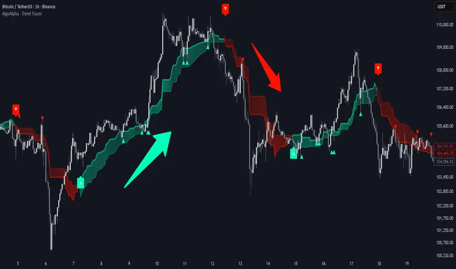
Trend Tracer [AlgoAlpha]🟠 OVERVIEW
This tool builds a two-stage trend model that reacts to structure shifts while also showing how strong or weak the move is. It uses a mid-price band (from the highest high and lowest low over a lookback) and applies two Supertrend passes on top of it. The first pass smoothens the basis. The second pass refines that direction and produces the final trail used for signals. A gradient fill between the two trails uses RSI of price-to-trail distance to show when price is stretched or cooling off. The aim is to give traders a simple way to read trend alignment, pressure, and early turns without guessing.
🟠 CONCEPTS
The script starts with a mid-range basis. This is the average of the rolling highest high and lowest low. It acts as a stable structure reference instead of raw close or typical price. From there, two Supertrend layers are applied:
• The first Supertrend uses a shorter ATR period and lower factor. It reacts faster and sets the main regime.
• The second Supertrend uses a slightly longer ATR and higher factor. It filters noise, waits for confirmed continuation, and generates the signal line.
The interaction between these trails matters. The outer Supertrend provides context by defining the broader regime. The inner Supertrend provides timing by flipping earlier and marking possible shifts. The gradient fill uses RSI of (close − supertrend value) to display when price stretches away from the trail. This shows strength, exhaustion, or compression within the trend.
🟠 FEATURES
Bullish and bearish flip markers placed at recent highs/lows
Rejection signals off the trend tracer line
Alerts for bullish and bearish trend changes
🟠 USAGE
Setup : Add the script to your chart. Timeframe is flexible; lower timeframes show more flips while higher ones give cleaner swings. Adjust Length to change how wide the basis range is. Use the two ATR settings and factors to match the volatility of the market you trade.
Read the chart : When the refined trail (stv_) sits above price the regime is bearish; when below, it is bullish. The wide trail (stv) confirms the larger move. Watch the gradient fill: darker colors appear when price is stretched from the trail and lighter colors appear when the move is weakening. Flip markers ▲ or ▼ highlight the first clean shift of the refined trail.
Settings that matter : Increasing the Main Factor slows main-trend flips and filters chop. Increasing the Signal Factor delays the timing trail but reduces noise. Shortening Length makes the basis more reactive. ATR periods change how sensitive each Supertrend pass is to volatility.
Bubbles + Clusters + SweepsIndicator For Bubbles + Clusters + Sweeps
✔ Volume bubbles
✔ Delta coloring (green/red intensity)
✔ Auto supply/demand zones
✔ Volume-profile style blocks inside zones
✔ Liquidity sweep markers
✔ Box drawings extending until filled
✔ Optional bubble filters (min-volume threshold)

Compression / ExpansionI created this Indicator to warn of compression and expansion so I could find the best area to trade I use it In conjunction with VWAP works on any timeframe and any asset where there is Volume
The Indicator produces a Letter C at the Start of Compression and a Letter E at the Start of Expansion you can change the settings to your liking On the chart my Expansion is in Red and compression is is Blue use In Conjunction with your favorite Indicators for Confluence
