Static Beta for Pair and Quant Trading A beta coefficient shows the volatility of an individual stock compared to the systematic risk of the entire market. Beta represents the slope of the line through a regression of data points. In finance, each point represents an individual stock's returns against the market.
Beta effectively describes the activity of a security's returns as it responds to swings in the market. It is used in the capital asset pricing model (CAPM), which describes the relationship between systematic risk and expected return for assets. CAPM is used to price risky securities and to estimate the expected returns of assets, considering the risk of those assets and the cost of capital.
Calculating Beta
A security's beta is calculated by dividing the product of the covariance of the security's returns and the market's returns by the variance of the market's returns over a specified period. The calculation helps investors understand whether a stock moves in the same direction as the rest of the market. It also provides insights into how volatile—or how risky—a stock is relative to the rest of the market.
For beta to provide useful insight, the market used as a benchmark should be related to the stock. For example, a bond ETF's beta with the S&P 500 as the benchmark would not be helpful to an investor because bonds and stocks are too dissimilar.
Beta Values
Beta equal to 1: A stock with a beta of 1.0 means its price activity correlates with the market. Adding a stock to a portfolio with a beta of 1.0 doesn’t add any risk to the portfolio, but it doesn’t increase the likelihood that the portfolio will provide an excess return.
Beta less than 1: A beta value less than 1.0 means the security is less volatile than the market. Including this stock in a portfolio makes it less risky than the same portfolio without the stock. Utility stocks often have low betas because they move more slowly than market averages.
Beta greater than 1: A beta greater than 1.0 indicates that the security's price is theoretically more volatile than the market. If a stock's beta is 1.2, it is assumed to be 20% more volatile than the market. Technology stocks tend to have higher betas than the market benchmark. Adding the stock to a portfolio will increase the portfolio’s risk, but may also increase its return.
Negative beta: A beta of -1.0 means that the stock is inversely correlated to the market benchmark on a 1:1 basis. Put options and inverse ETFs are designed to have negative betas. There are also a few industry groups, like gold miners, where a negative beta is common.
LET'S START
Now I'll give my own definition.
Beta:
If we assume market caps are equal ,
it is an indicator that shows how much of the second instrument we should buy if we buy one of the first, taking into account the price volatility of two instruments.
But if the market caps are not equal:
For example, the ETF for A is $300.
The ETF for B is $600.
If static beta predicted by this script is 0.5:
300 * 1 * a = 600 * 0.5 * b
Then we should use 1 b for 1 a.
(Long a and short b or vice versa )
So, we can try pair trading for a/b or a-b.
However, these values are generally close to each other, such as 0.8 and 0.93. However, the closer we can adjust our lot purchases to bring the double beta to a value closer to 1, the higher the hedge ratio will be.
Large commercials use dynamic betas, which are updated periodically, in addition to static betas
However, scaling this is very difficult for individual investors with limited investment tools.
But a static beta of 5,000 bars is still much better than not considering any beta at all.
Note: The presence of a beta value for two instruments does not necessarily mean they can be included in pair trading.
It is also important (%99) to consider historically very high correlations and cointegration relationships, as well as the compatibility of security structures.
Note 2 : This script is designed for low timeframes.
Do not use betas from different timeframes.
Beta dynamics are different for each timeframe.
Note 3 : I created this script with the help of ChatGPT.
Source for beta definition ( ) :
www.investopedia.com
Regards.
Statistics

Breakouts & Pullbacks [Trendoscope®]🎲 Breakouts & Pullbacks - All-Time High Breakout Analyzer
Probability-Based Post-Breakout Behavior Statistics | Real-Time Pullback & Runup Tracker
A professional-grade Pine Script v6 indicator designed specifically for analyzing the historical and real-time behavior of price after strong All-Time High (ATH) breakouts. It automatically detects significant ATH breakouts (with configurable minimum gap), measures the depth and duration of pullbacks, the speed of recovery, and the subsequent run-up strength — then turns all this data into easy-to-read statistical probabilities and percentile ranks.
Perfect for swing traders, breakout traders, and anyone who wants objective, data-driven insight into questions like:
“How deep do pullbacks usually get after a strong ATH breakout?”
“How many bars does it typically take to recover the breakout level?”
“What is the median run-up after recovery?”
“Where is the current pullback or run-up relative to historical ones?”
🎲 Core Concept & Methodology
Indicator is more suitable for indices or index ETFs that generally trade in all-time highs however subjected to regular pullbacks, recovery and runups.
For every qualified ATH breakout, the script identifies 4 distinct phases:
Breakout Point – The exact bar where price closes above the previous ATH after at least Minimum Gap bars.
Pullback Phase – From breakout candle high → lowest low before price recovers back above the breakout level.
Recovery Phase – From the pullback low → the bar where price first trades back above the original breakout price.
Post-Recovery Run-up Phase – From the recovery point → current price (or highest high achieved so far).
Each completed cycle is stored permanently and used to build a growing statistical database unique to the loaded chart and timeframe.
🎲 Visual Elements
Yellow polyline triangle connecting Previous ATH / Pullback point(start), New ATH Breakout point (end), Recovery point (lowest pullback price), and extends to recent ATH price.
Small green label at the pullback low showing detailed tooltip on hover with all measured values
Clean, color-coded statistics table in the top-right corner (visible only on the last bar)
Powerful Statistics Table – The Heart of the Indicator
The table constantly compares the current situation against all past qualified breakouts and shows details about pullbacks, and runups that help us calculate the probability of next pullback, recovery or runup.
🎲 Settings & Inputs
Minimum Gap
The minimum number of bars that must pass between breaking a new ATH and the previous one.
Higher values = stricter filter → only the strongest, cleanest breakouts are counted.
Lower values = more data points (useful on lower timeframes or very trending instruments).
Recommendation:
Daily charts: 30–50
4H charts: 40–80
1H charts: 100–200
🎲 How to Use It in Practice
This indicator helps investors to understand when to be bullish, bearish or cautious and anticipate regular pullbacks, recovery of markets using quantitative methods.
The indicator does not generate buy/sell signals. However, helps traders set expectations and anticipate market movements based on past behavior.

Last CLOSED Bar OHLCThis TradingView Pine Script (@version=6) creates a label that displays the previous fully closed candlestick’s OHLC data on the chart.

Bitcoin vs M2 Global Liquidity (Lead 3M) - Table Ticker═══════════════════════════════════════════════════════════════
Bitcoin vs M2 Global Liquidity - Regression Indicator
═══════════════════════════════════════════════════════════════
TECHNICAL SPECS
• Pine Script v6
• Overlay: false (separate pane)
• Data sources: 5 M2 series + 4 FX pairs (request.security)
• Calculation: Rolling OLS linear regression with configurable lead
• Output: Regression line + ±1σ/±2σ confidence bands + R² ticker
CORE FUNCTIONALITY
Aggregates M2 money supply from 5 central banks (CN, US, EU, JP, GB),
converts to USD, applies time-lead, runs rolling linear regression
vs Bitcoin price, plots predicted value with confidence intervals.
CONFIGURABLE PARAMETERS
Input Controls:
• Lead Period: 0-365 days (default: 90)
• Lookback Window: 50-2000 bars (default: 750)
• Bands: Toggle ±1σ and ±2σ visibility
• Colors: BTC, M2, regression line, confidence zones
• Ticker: Position, size, colors, transparency
Advanced Settings:
• Table display: R², lead, M2 total, country breakdown (%)
• Ticker customization: 9 position options, 6 text sizes
• Border: Width 0-10px, color, outline-only mode
DATA AGGREGATION
Sources (via request.security):
• ECONOMICS:CNM2, USM2, EUM2, JPM2, GBM2
• FX_IDC:CNYUSD, JPYUSD (others: FX:EURUSD, GBPUSD)
• Conversion: All M2 → USD → Sum / 1e12 (trillions)
REGRESSION ENGINE
• Arrays: m2Array, btcArray (dynamic sizing, auto-trim)
• Window: Rolling (lookbackPeriod bars)
• Lead: Time-shift via array indexing (i + leadPeriodDays)
• Calc: Manual OLS (covariance/variance), no built-in ta functions
• Outputs: slope, intercept, r2, stdResiduals
CONFIDENCE BANDS
±1σ and ±2σ calculated from standard deviation of residuals.
Fill zones between upper/lower bounds with configurable transparency.
ALERTS
5 pre-configured alertcondition():
• Divergence > 15%
• Price crosses ±1σ bands (up/down)
• Price crosses ±2σ bands (up/down)
TICKER TABLE
Dynamic table.new() with 9 rows:
• R² value (4 decimals)
• Lead period (days + months)
• M2 Global total (trillions USD)
• Country breakdown: CN, US, EU, JP, GB (absolute + %)
• Optional: Hide/show M2 details
VISUAL CUSTOMIZATION
All plot() elements support:
• Color picker inputs (group="Couleurs")
• Line width: 1-3px
• Transparency: 0-100% for zones
• Offset: M2 plot has +leadPeriodDays offset option
PERFORMANCE
• Max arrays size: lookbackPeriod + leadPeriodDays + 200
• Calculations: Only when array.size >= lookbackPeriod + leadPeriodDays
• Table update: barstate.islast (once per bar)
• Request.security: gaps_off mode
CODE STRUCTURE
1. Inputs (lines 7-54)
2. Data fetch (lines 56-76)
3. M2 aggregation (line 78)
4. Array management (lines 84-95)
5. Regression calc (lines 97-172)
6. Prediction + bands (lines 174-183)
7. Plots (lines 185-199)
8. Ticker table (lines 201-236)
9. Alerts (lines 238-246)
DEPENDENCIES
None. Pure Pine Script v6. No external libraries.
LIMITATIONS
• Daily timeframe recommended (1D)
• Requires 750+ bars history for optimal calculation
• M2 data availability: TradingView ECONOMICS feed
• Max lines: 500 (declared in indicator())
CUSTOMIZATION EXAMPLES
• Shorter lookback (200d): More reactive, lower R²
• Longer lookback (1500d): More stable, regime mixing
• No bands: Set showBands=false for clean view
• Different lead: Test 60d, 120d for sensitivity analysis
TECHNICAL NOTES
• Manual OLS implementation (no ta.linreg)
• Array-based lead application (not plot offset)
• M2 values stored in trillions (/ 1e12) for readability
• Residuals array cleared/rebuilt each calculation
OPEN SOURCE
Code fully visible. Modify, fork, analyze freely.
No hidden calculations. No proprietary data.
VERSION
1.0 | November 2025 | Pine Script v6
═══════════════════════════════════════════════════════════════

High Volume Bars (Advanced)High Volume Bars (Advanced)
High Volume Bars (Advanced) is a Pine Script v6 indicator for TradingView that highlights bars with unusually high volume, with several ways to define “unusual”:
Classic: volume > moving average + N × standard deviation
Change-based: large change in volume vs previous bar
Z-score: statistically extreme volume values
Robust mode (optional): median + MAD, less sensitive to outliers
It can:
Recolor candles when volume is high
Optionally highlight the background
Optionally plot volume bands (center ± spread × multiplier)
⸻
1. How it works
At each bar the script:
Picks the volume source:
If Use Volume Change vs Previous Bar? is off → uses raw volume
If on → uses abs(volume - volume )
Computes baseline statistics over the chosen source:
Lookback bars
Moving average (SMA or EMA)
Standard deviation
Optionally replaces mean/std with robust stats:
Center = median (50th percentile)
Spread = MAD (median absolute deviation, scaled to approx σ)
Builds bands:
upper = center + spread * multiplier
lower = max(center - spread * multiplier, 0)
Flags a bar as “high volume” if:
It passes the mode logic:
Classic abs: volume > upper
Change mode: abs(volume - volume ) > upper
Z-score mode: z-score ≥ multiplier
AND the relative filter (optional): volume > average_volume * Min Volume vs Avg
AND it is past the first Skip First N Bars from the start of the chart
Colors the bar and (optionally) the background accordingly.
⸻
2. Inputs
2.1. Statistics
Lookback (len)
Number of bars used to compute the baseline stats (mean / median, std / MAD).
Typical values: 50–200.
StdDev / Z-Score Multiplier (mult)
How far from the baseline a bar must be to count as “high volume”.
In classic mode: volume > mean + mult × std
In z-score mode: z ≥ mult
Typical values: 1.0–2.5.
Use EMA Instead of SMA? (smooth_with_ema)
Off → uses SMA (slower but smoother).
On → uses EMA (reacts faster to recent changes).
Use Robust Stats (Median & MAD)? (use_robust)
Off → mean + standard deviation
On → median + MAD (less sensitive to a few insane spikes)
Useful for assets with occasional volume blow-ups.
⸻
2.2. Detection Mode
These inputs control how “unusual” is defined.
• Use Volume Change vs Previous Bar? (mode_change)
• Off (default) → uses absolute volume.
• On → uses abs(volume - volume ).
You then detect jumps in volume rather than absolute size.
Note: This is ignored if Z-Score mode is switched on (see below).
• Use Z-Score on Volume? (Overrides change) (mode_zscore)
• Off → high volume when raw value exceeds the upper band.
• On → computes z-score = (value − center) / spread and flags a bar as high when z ≥ multiplier.
Z-score mode can be combined with robust stats for more stable thresholds.
• Min Volume vs Avg (Filter) (min_rel_mult)
An extra filter to ignore tiny-volume bars that are statistically “weird” but not meaningful.
• 0.0 → no filter (all stats-based candidates allowed).
• 1.0 → high-volume bar must also be at least equal to average volume.
• 1.5 → bar must be ≥ 1.5 × average volume.
• Skip First N Bars (from start of chart) (skip_open_bars)
Skips the first N bars of the chart when evaluating high-volume conditions.
This is mostly a safety / cosmetic option to avoid weird behavior on very early bars or backfill.
⸻
2.3. Visuals
• Show Volume Bands? (show_bands)
• If on, plots:
• Upper band (upper)
• Lower band (lower)
• Center line (vol_center)
These are plotted on the same pane as the script (usually the price chart).
• Also Highlight Background? (use_bg)
• If on, fills the background on high-volume bars with High-Vol Background.
• High-Vol Bar Transparency (0–100) (bar_transp)
Controls the opacity of the high-volume bar colors (up / down).
• 0 → fully opaque
• 100 → fully transparent (no visible effect)
• Up Color (upColor) / Down Color (dnColor)
• Regular bar colors (non high-volume) for up and down bars.
• Up High-Vol Base Color (upHighVolBase) / Down High-Vol Base Color (dnHighVolBase)
Base colors used for high-volume up/down bars. Transparency is applied on top of these via bar_transp.
• High-Vol Background (bgHighVolColor)
Background color used when Also Highlight Background? is enabled.
⸻
3. What gets colored and how
• Bar color (barcolor)
• Up bar:
• High volume → Up High-Vol Color
• Normal volume → Up Color
• Down bar:
• High volume → Down High-Vol Color
• Normal volume → Down Color
• Flat bar → neutral gray
• Background color (bgcolor)
• If Also Highlight Background? is on, high-volume bars get High-Vol Background.
• Otherwise, background is unchanged.
⸻
4. Alerts
The indicator exposes three alert conditions:
• High Volume Bar
Triggers whenever is_high is true (up or down).
• High Volume Up Bar
Triggers only when is_high is true and the bar closed up (close > open).
• High Volume Down Bar
Triggers only when is_high is true and the bar closed down (close < open).
You can use these in TradingView’s “Create Alert” dialog to:
• Get notified of potential breakout / exhaustion bars.
• Trigger webhook events for bots / custom infra.
⸻
5. Recommended presets
5.1. “Classic” high-volume detector (closest to original)
• Lookback: 150–200
• StdDev / Z-Score Multiplier: 1.0–1.5
• Use EMA Instead of SMA?: off
• Use Robust Stats?: off
• Use Volume Change vs Previous Bar?: off
• Use Z-Score on Volume?: off
• Min Volume vs Avg (Filter): 0.0–1.0
Behavior: Flags bars whose volume is notably above the recent average (plus a bit of noise filtering), same spirit as your initial implementation.
⸻
5.2. Volatility-aware (Z-score) mode
• Lookback: 100–200
• StdDev / Z-Score Multiplier: 1.5–2.0
• Use EMA Instead of SMA?: on
• Use Robust Stats?: on (if asset has huge spikes)
• Use Volume Change vs Previous Bar?: off (ignored anyway in z-score mode)
• Use Z-Score on Volume?: on
• Min Volume vs Avg (Filter): 0.5–1.0
Behavior: Flags bars that are “statistically extreme” relative to recent volume behavior, not just absolutely large. Good for assets where baseline volume drifts over time.
⸻
5.3. “Wake-up bar” (volume acceleration)
• Lookback: 50–100
• StdDev / Z-Score Multiplier: 1.0–1.5
• Use EMA Instead of SMA?: on
• Use Robust Stats?: optional
• Use Volume Change vs Previous Bar?: on
• Use Z-Score on Volume?: off
• Min Volume vs Avg (Filter): 0.5–1.0
Behavior: Emphasis on sudden increases in volume rather than absolute size – useful to catch “first active bar” after a quiet period.
⸻
6. Limitations / notes
• Time-of-day effects
The script currently treats the entire chart as one continuous “session”. On 24/7 markets (crypto) this is fine. For regular-session assets (equities, futures), volume naturally spikes at open/close; you may want to:
• Use a shorter Lookback, or
• Add a session-aware filter in a future iteration.
• Illiquid symbols
On very low-liquidity symbols, robust stats (Use Robust Stats) and a non-zero Min Volume vs Avg can help avoid “everything looks extreme” problems.
• Overlay behavior
overlay = true means:
• Bars are recolored on the price pane.
• Volume bands are also drawn on the price pane if enabled.
If you want a dedicated panel for the bands, duplicate the logic in a separate script with overlay = false.

Reversal Correlation Pressure [OmegaTools]Reversal Correlation Pressure is a quantitative regime-detection and signal-filtering framework designed to enhance both reversal timing and breakout validation across intraday and multi-session markets.
It is built for discretionary and systematic traders who require a statistically grounded filter capable of adapting to changing market conditions in real time.
1. Purpose and Overview
Market conditions constantly rotate through phases of expansion, contraction, trend persistence, and noise-driven mean reversion. Many strategies break down not because the signal is wrong, but because the regime is unsuitable.
This indicator solves that structural problem.
The tool measures the evolving correlation relationship between highs and lows — a robust proxy for how “organized” or “fragmented” price discovery currently is — and transforms it into a regime pressure reading. This reading is then used as the core variable to validate or filter reversal and breakout opportunities.
Combined with an internal performance-based filter that learns from its past signals, the indicator becomes a dynamic decision engine: it highlights only the signals that statistically perform best under the current market regime.
2. Core Components
2.1 Correlation-Based Regime Mapping
The relationship between highs and lows contains valuable information about market structure:
High correlation generally corresponds to coherent, directional markets where momentum and breakouts tend to prevail.
Low or unstable correlation often appears in overlapping, rotational phases where price oscillates and mean-reversion behavior dominates.
The indicator continuously evaluates this correlation, normalizes it statistically, and displays it as a pressure histogram:
Higher values indicate regimes favorable to trend continuation or momentum breakouts.
Lower values indicate regimes where reversals, pullbacks, and fade setups historically perform better.
This regime mapping is the foundation upon which the adaptive filter operates.
2.2 Reversal Stress & Breakout Stress Signaling
Raw directional opportunities are identified using statistically significant deviations from short-term equilibrium (overbought/oversold dynamics).
However, unlike traditional mean-reversion or breakout tools, signals here are not automatically taken. They must first be validated by the regime framework and then compared against the performance of similar past setups.
This dual evaluation sharply reduces the noise associated with reversal attempts during strong trends, while also preventing breakout attempts during choppy, anti-directional conditions.
2.3 Adaptive Regime-Selection Backtester
A key innovation of this indicator is its embedded micro-backtester, which continuously tracks how reversal or breakout signals have performed under each correlation regime.
The system evaluates two competing hypotheses:
Signals perform better during high-correlation regimes.
Signals perform better during low-correlation or neutral regimes.
For each new trigger, the indicator looks back at a rolling sample of past setups and measures short-term performance under both regimes. It then automatically selects the regime that currently demonstrates the superior historical edge.
In other words, the indicator:
Learns from recent market behavior
Determines which regime supports reversals
Determines which regime supports breakouts
Applies the optimal filter in real time
Highlights only the signals that historically outperformed under similar conditions
This creates a dynamic, statistically supervised approach to signal filtering — a substantial improvement over static or fixed-threshold systems.
2.4 Visual Components
To support rapid decision-making:
Correlation Pressure Histogram:
Encodes regime strength through a gradient-based color system, transitioning from neutral contexts into strong structural phases.
Directional Markers:
Visual arrows appear when a signal passes all filters and conditions.
Bar Coloring:
Bars can optionally be recolored to reflect active bullish or bearish bias after the adaptive filter approves a signal.
These components integrate seamlessly to give the trader a concise but complete view of the underlying conditions.
3. How to Use This Indicator
3.1 Identifying Regimes
The histogram is the anchor:
High, brightly colored columns suggest trend-friendly behavior where breakout alignment and directional follow-through have historically been stronger.
Low or muted columns suggest mean-reversion contexts where counter-trend opportunities and reversal setups gain reliability.
3.2 Filtering Signals
The indicator automatically decides whether a reversal or breakout trigger should be respected based on:
the current correlation regime,
the learned performance of recent signals under similar conditions, and
the directional stress detected in price.
The user does not need to adjust anything manually.
3.3 Integration with Other Tools
This indicator works best when combined with:
VWAP or session levels
Market internals and breadth metrics
Volume, order flow, or delta-based tools
Local structural frameworks (support/resistance, liquidity highs and lows)
Its strength is in telling you when your other signals matter and when they should be ignored.
4. Strengths of the Framework
Automatically adapts to changing micro-regimes
Reduces false reversals during strong trends
Avoids false breakouts in overlapping, rotational markets
Learns from recent historical performance
Provides a statistically driven confirmation layer
Works on all liquid assets and timeframes
Suitable for both discretionary and automated environments
5. Disclaimer
This indicator is provided strictly for educational and analytical purposes.
It does not constitute trading advice, investment guidance, or a recommendation to buy or sell any financial instrument.
Past performance of any statistical filter or adaptive method does not guarantee future results.
All trading involves significant risk, and users are responsible for their own decisions and risk management.
By using this indicator, you acknowledge that you are fully responsible for your trading activity.

Spot-Futures SpreadSpot-Futures Spread Indicator
A comprehensive indicator that automatically calculates and visualizes the percentage spread between spot and perpetual futures prices across multiple exchanges.
Key Features:
Automatic Exchange Detection - Automatically detects your current exchange and finds the corresponding spot/futures pair
Smart Fallback System - If the counterpart isn't available on your exchange, it automatically searches across 7+ major exchanges (Binance, Bybit, OKX, Gate.io, MEXC, KuCoin, HTX) and uses the first valid match
Multi-Exchange Support - Works with 14 exchanges including Binance, Bybit, OKX, MEXC, BitGet, Gate.io, KuCoin, and more
Clear Exchange Attribution - Shows exactly which exchanges are providing spot and futures data in the statistics table
Configurable Moving Average - Track the average spread with customizable period
Standard Deviation Bands - Identify unusual spread conditions with Bollinger-style bands
Built-in Alerts - Get notified when spread crosses bands or zero (parity)
Statistics Table - Real-time stats showing current spread, MA, std dev, and bands
Manual Override Options - Advanced users can manually specify exchanges and symbols
How It Works:
The indicator calculates the spread as: (Futures Price - Spot Price) / Spot Price × 100
Positive spread = Futures trading at a premium (contango)
Negative spread = Futures trading at a discount (backwardation)
Zero = Parity between spot and futures
Use Cases:
Funding Rate Analysis - Correlates with perpetual funding rates
Arbitrage Opportunities - Identify significant spot-futures divergences
Market Sentiment - Premium/discount indicates bullish/bearish positioning
Cross-Exchange Analysis - Compare spreads when spot and futures are on different exchanges
Smart Features:
Works whether you're viewing a spot or futures chart
Automatically handles exchange-specific perpetual contract naming (.P, PERP, SWAP, etc.)
Color-coded visualization (green for premium, red for discount)
Customizable colors and display options
Background shading based on spread direction
Perfect For:
Crypto traders monitoring funding rates, arbitrage traders, market makers, and anyone interested in spot-futures dynamics across multiple exchanges.
Getting Started:
Simply add the indicator to any spot or perpetual futures chart. It will automatically detect the exchange and find the corresponding pair. The statistics table shows which exchanges are being used for maximum transparency.
Note: The indicator automatically ignores invalid symbols, so you'll never see errors even if a specific pair doesn't exist on a particular exchange.
Kudos to @AlekMel that made the "Spot - Fut Spread v2" indicator that I enhance the Automatic detection feature which was not working in some case.

Stochastic Ensembling of OutputsStochastic Ensembling of Outputs
🙏🏻 This is a simple tool/method that would solve naturally many well known problems:
“Price reversed 1 tick before the actual level, not executing my limit order”
“I consider intraday trend change by checking whether price is above/below VWAP, but is 1 tick enough? What to do, price is now whipsawing around vwap...”.
“I want to gradually accumulate a position around a chosen anchor. But where exactly should I put my orders? And I want to automate it ofc.“
“All these DSP adepts are telling you about some kind of noise in the markets… But how can I actually see it?”
The easy fix is to make things more analog less digital, by synthesizing numerous noise instances & adding it to any price-applied metric of yours. The ones who fw techno & psytrance, and other music, probably don’t need any more explanations. Then by checking not just 2 lines or 1 process against another one, you will be checking cloud vs cloud of lines, even allowing you to introduce proxies of probabilities. More crosses -> more confirmation to act.
How-to use:
The tool has 2 inputs: source and target:
Sources should always be the underlying process. If you apply the tool to price based metric, leave it hlcc4 unless you have a better one point estimate for each bar;
Target is your target, e.g if you want to apply it to VWAP, pick VWAP as target. You can thee on the chart above how trading activity recently never exactly touched VWAP, however noised instances of VWAP 'were' touched
The code is clean and written in modular form, you can simply copy paste it to any script of yours if you don't want to have multiple study-on-study script pairs.
^^ applied to prev days highs and lows
^^ applied to MBAD extensions and basis
^^ applied to input series itself
Here’s how it works, no ML, no “AI”, no 1k lines of code, just stats:
The problem with metrics, even if they are time aware like WMA, is that they still do not directly gain information about “changes” between datapoints. If we pick noise characteristics to match these changes, we’d effectively introduce this info into our ops.
^^ this screenshot represents 2 very different processes: a sine wave and white noise, see how the noise instances learned from each process differ significantly.
Changes can be represented as AR1 process . It’s dead simple, no PHD needed, it’s just how the current datapoint is related (or not) to the previous datapoint, no more than 1, and how this relationship holds/evolves over time. Unlike the mainstream approach like MLE, I estimate this relationship (phi parameter) via MoM but giving more weights to more recent datapoints via exponential smoothing over all the data available on your charts (so I encode temporal information), algocomplexity is O(1), lighting fast, just one pass. <- that gives phi , we’d use it as color for our noise generator
Then we just need to estimate noise amplitude ( gamma ) via checking what AR1 model actually thought vs the reality, variance of these innovations. Same via exponential smoothing, time aware, O(1), one pass, it’s all it does.
Then we generate white gaussian noise, and apply 2 estimated parameters (phi and gamma), and that’s all.
Omg, I think I just made my first real DSP script xd
Just like Monte Carlo for risk management, this is so simple and natural I can’t believe so many “pros” hide it and never talk about it in open access. Sharing it here on TradingView would’ve not done anything critical for em, but many would’ve benefited.
∞

Global M2 Money Supply Growth (GDP-Weighted)📊 Global M2 Money Supply Growth (GDP-Weighted)
This indicator tracks the weighted aggregate M2 money supply growth across the world's four largest economies: United States, China, Eurozone, and Japan. These economies represent approximately 69.3 trillion USD in combined GDP and account for the majority of global liquidity, making this a comprehensive macro indicator for analyzing worldwide monetary conditions.
════════════════════════════════════════════
🔧 KEY FEATURES:
📈 GDP-Weighted Aggregation
Each economy is weighted proportionally by its nominal GDP using 2025 IMF World Economic Outlook data:
• United States: 44.2% (30.62 trillion USD)
• China: 28.0% (19.40 trillion USD)
• Eurozone: 21.6% (15.0 trillion USD)
• Japan: 6.2% (4.28 trillion USD)
The weights are fully adjustable through the indicator settings, allowing you to update them annually as new IMF forecasts are released (typically April and October).
⏱️ Multiple Time Period Options
Choose between three calculation methods to analyze different timeframes:
• YoY (Year-over-Year): 12-month growth rate for identifying long-term liquidity trends and cycles
• MoM (Month-over-Month): 1-month growth rate for detecting short-term monetary policy shifts
• QoQ (Quarter-over-Quarter): 3-month growth rate for medium-term trend analysis
🔄 Advanced Offset Function
Shift the entire indicator forward by 0-365 days to test lead/lag relationships between global liquidity and asset prices. Research suggests a 56-70 day lag between M2 changes and Bitcoin price movements, but you can experiment with different offsets for various assets (equities, gold, commodities, etc.).
🌍 Individual Country Breakdown
Real-time display of each economy's M2 growth rate with:
• Current percentage change (YoY/MoM/QoQ)
• GDP weight contribution
• Color-coded values (green = monetary expansion, red = contraction)
📊 Smart Overlay Capability
Displays directly on your main price chart with an independent left-side scale, allowing you to visually correlate global liquidity trends with any asset's price action without cluttering the chart.
🔧 Customizable GDP Weights
All GDP values can be adjusted through the indicator settings without editing code, making annual updates simple and accessible for all users.
════════════════════════════════════════════
📡 DATA SOURCES:
All M2 money supply data is sourced from ECONOMICS (Trading Economics) for consistency and reliability:
• ECONOMICS:USM2 (United States)
• ECONOMICS:CNM2 (China)
• ECONOMICS:EUM2 (Eurozone)
• ECONOMICS:JPM2 (Japan)
All values are normalized to USD using current daily exchange rates (USDCNY, EURUSD, USDJPY) before GDP-weighted aggregation, ensuring accurate cross-country comparisons.
══════════════════════════════════════════════
💡 USE CASES & APPLICATIONS:
🔹 Liquidity Cycle Analysis
Track global monetary expansion/contraction cycles to identify when central banks are coordinating loose or tight monetary policies.
🔹 Market Timing & Risk Assessment
High M2 growth (>10%) historically correlates with risk-on environments and rising asset prices across crypto, equities, and commodities. Negative M2 growth signals monetary tightening and potential market corrections.
🔹 Bitcoin & Crypto Correlation
Compare with Bitcoin price using the offset feature to identify the optimal lag period. Many traders use 60-70 day offsets to predict crypto market movements based on liquidity changes.
🔹 Macro Portfolio Allocation
Use as a regime filter to adjust portfolio exposure: increase risk assets during liquidity expansion, reduce during contraction.
🔹 Central Bank Policy Divergence
Monitor individual country metrics to identify when major central banks are pursuing divergent policies (e.g., Fed tightening while China eases).
🔹 Inflation & Economic Forecasting
Rapid M2 growth often leads inflation by 12-18 months, making this a leading indicator for future inflation trends.
🔹 Recession Early Warning
Negative M2 growth is extremely rare and has preceded major recessions, making this a valuable risk management tool.
════════════════════════════════════════════
📊 INTERPRETATION GUIDE:
🟢 +10% or Higher
Aggressive monetary expansion, typically during crises (2001, 2008, 2020). The COVID-19 period saw M2 growth reach 20-27%, which preceded significant inflation and asset price surges. Strong bullish signal for risk assets.
🟢 +6% to +10%
Above-average liquidity growth. Central banks are providing stimulus beyond normal levels. Generally favorable for equities, crypto, and commodities.
🟡 +3% to +6%
Normal/healthy growth rate, roughly in line with GDP growth plus 2% inflation targets. Neutral environment with moderate support for risk assets.
🟠 0% to +3%
Slowing liquidity, potential tightening phase beginning. Central banks may be raising rates or reducing balance sheets. Caution warranted for high-beta assets.
🔴 Negative Growth
Monetary contraction - extremely rare. Only occurred during aggressive Fed tightening in 2022-2023. Strong warning signal for risk assets, often precedes recessions or major market corrections.
════════════════════════════════════════════
🎯 OPTIMAL USAGE:
📅 Recommended Timeframes:
• Daily or Weekly charts for macro analysis
• Monthly charts for very long-term trends
💹 Compatible Asset Classes:
• Cryptocurrencies (especially Bitcoin, Ethereum)
• Equity indices (S&P 500, NASDAQ, global markets)
• Commodities (Gold, Silver, Oil)
• Forex majors (DXY correlation analysis)
⚙️ Suggested Settings:
• Default: YoY calculation with 0 offset for current liquidity conditions
• Bitcoin traders: YoY with 60-70 day offset for predictive analysis
• Short-term traders: MoM with 0 offset for recent policy changes
• Quarterly rebalancers: QoQ with 0 offset for medium-term trends
════════════════════════════════════════════
📋 VISUAL DISPLAY:
The indicator plots a blue line showing the selected growth metric (YoY/MoM/QoQ), with a dashed reference line at 0% to clearly identify expansion vs. contraction regimes.
A comprehensive table in the top-right corner displays:
• Current global M2 growth rate (large, prominent display)
• Individual country breakdowns with their GDP weights
• Color-coded growth rates (green for positive, red for negative)
════════════════════════════════════════════
🔄 MAINTENANCE & UPDATES:
GDP weights should be updated annually (ideally in April or October) when the IMF releases new World Economic Outlook forecasts. Simply adjust the four GDP input parameters in the indicator settings - no code editing required.
The relative GDP proportions between the Big 4 economies change very gradually (typically <1-2% per year), so even if you update weights once every 1-2 years, the impact on the indicator's accuracy is minimal.
════════════════════════════════════════════
💭 TRADING PHILOSOPHY:
This indicator embodies the principle that "liquidity drives markets." By tracking the combined M2 money supply of the world's largest economies, weighted by their economic size, you gain insight into the fundamental liquidity conditions that underpin all asset prices.
Unlike single-country M2 indicators, this GDP-weighted approach captures the true global picture, accounting for the fact that US monetary policy has 2x the impact of Japanese policy due to economic size differences.
Perfect for macro-focused traders, long-term investors, and anyone seeking to understand the "tide that lifts all boats" in financial markets.
════════════════════════════════════════════
Created for traders and investors who incorporate global liquidity trends into their decision-making process. Best used alongside other technical and fundamental analysis tools for comprehensive market assessment.
⚠️ Disclaimer: M2 money supply is a lagging macroeconomic indicator. Past correlations do not guarantee future results. Always use proper risk management and combine with other analysis methods.

Mean Reversion Signals (v6.4) – VWAP ±SD use with "support and resistence levels with breaks {lux algo} " at 5m tf for better results

Price Drop CounterThe Price Drop Counter is a very basic statistical indicator.
See it as an analytical tool that tracks how many times an asset's price has dropped by a specified percentage from its recent peak within a defined date range.
The indicator monitors the highest price reached and counts each occurrence when the price falls by your chosen threshold, then resets its peak tracking point after each drop is registered.
Uses
Volatility Assessment: Measure how frequently significant price corrections occur during specific periods
Market Behavior Analysis: Compare drop frequency across different timeframes or market conditions
Risk Evaluation: Identify assets or periods with higher downside volatility
Historical Pattern Recognition: Study how often major pullbacks happened during bull or bear markets
Backtesting Support: Analyze how your strategy would perform based on the frequency of drawdowns
How to use it
Add the indicator to your TradingView chart
Configure the Percent Drop (%) to define your threshold (default: 10%). The indicator will count each time price falls by this percentage from the most recent high
IMPORTANT Set your Start Date and End Date to analyze a specific period of interest
The blue step-line plot shows the cumulative count of drops within your date range
Adjust the percentage threshold based on your analysis needs - use smaller values (2-5%) for more frequent signals or larger values (15-20%) for major corrections only
The counter resets its high-water mark after each qualifying drop, allowing it to track multiple sequential drops within the same period.

indicator CalibrationIndicator Calibration - Multi-Indicator Consensus System
Overview
Indicator Calibration is a powerful consensus-based trading indicator that leverages the MyIndicatorLibrary (NormalizedIndicators) to combine multiple trend-following indicators into a single, actionable signal. By averaging the normalized outputs of up to 8 different trend indicators, this tool provides traders with a clear consensus view of market direction, reducing noise and false signals inherent in single-indicator approaches.
The indicator outputs a value between -1 (strong bearish) and +1 (strong bullish), with 0 representing a neutral market state. This creates an intuitive, easy-to-read oscillator that synthesizes multiple analytical perspectives into one coherent signal.
🎯 Core Concept
Consensus Trading Philosophy
Rather than relying on a single indicator that may give conflicting or premature signals, Indicator Calibration employs a democratic voting system where multiple indicators contribute their normalized opinion:
Each enabled indicator votes: +1 (bullish), -1 (bearish), or 0 (neutral)
The votes are averaged to create a consensus signal
Strong consensus (closer to ±1) indicates high agreement among indicators
Weak consensus (closer to 0) indicates market indecision or transition
Key Benefits
Reduced False Signals: Multiple indicators must agree before strong signals appear
Noise Filtering: Individual indicator quirks are smoothed out by averaging
Customizable: Enable/disable indicators and adjust parameters to suit your trading style
Universal Application: Works across all timeframes and asset classes
Clear Visualization: Simple line oscillator with clear bull/bear zones
📊 Included Indicators
The system can utilize up to 8 normalized trend-following indicators from the library:
1. BBPct - Bollinger Bands Percent
Parameters: Length (default: 20), Factor (default: 2)
Type: Stationary oscillator
Strength: Mean reversion and volatility detection
2. NorosTrendRibbonEMA
Parameters: Length (default: 20)
Type: Non-stationary trend follower
Strength: Breakout detection with momentum confirmation
3. RSI - Relative Strength Index
Parameters: Length (default: 9), SMA Length (default: 4)
Type: Stationary momentum oscillator
Strength: Overbought/oversold with smoothing
4. Vidya - Variable Index Dynamic Average
Parameters: Length (default: 30), History Length (default: 9)
Type: Adaptive moving average
Strength: Volatility-adjusted trend following
5. HullSuite
Parameters: Length (default: 55), Multiplier (default: 1)
Type: Fast-response moving average
Strength: Low-lag trend identification
6. TrendContinuation
Parameters: MA Length 1 (default: 50), MA Length 2 (default: 25)
Type: Dual HMA system
Strength: Trend quality assessment with neutral states
7. LeonidasTrendFollowingSystem
Parameters: Short Length (default: 21), Key Length (default: 10)
Type: Dual EMA crossover
Strength: Simple, reliable trend tracking
8. TRAMA - Trend Regularity Adaptive Moving Average
Parameters: Length (default: 50)
Type: Adaptive trend follower
Strength: Adjusts to trend stability
⚙️ Input Parameters
Source Settings
Source: Choose your price input (default: close)
Can be modified to: open, high, low, close, hl2, hlc3, ohlc4, hlcc4
Indicator Selection
Each indicator can be enabled or disabled via checkboxes:
use_bbpct: Enable/disable Bollinger Bands Percent
use_noros: Enable/disable Noro's Trend Ribbon
use_rsi: Enable/disable RSI
use_vidya: Enable/disable VIDYA
use_hull: Enable/disable Hull Suite
use_trendcon: Enable/disable Trend Continuation
use_leonidas: Enable/disable Leonidas System
use_trama: Enable/disable TRAMA
Parameter Customization
Each indicator has its own parameter group where you can fine-tune:
val 1: Primary period/length parameter
val 2: Secondary parameter (multiplier, smoothing, etc.)
📈 Signal Interpretation
Output Line (Orange)
The main output oscillates between -1 and +1:
+1.0 to +0.5: Strong bullish consensus (all or most indicators agree on uptrend)
+0.5 to +0.2: Moderate bullish bias (bullish indicators outnumber bearish)
+0.2 to -0.2: Neutral zone (mixed signals or transition phase)
-0.2 to -0.5: Moderate bearish bias (bearish indicators outnumber bullish)
-0.5 to -1.0: Strong bearish consensus (all or most indicators agree on downtrend)
Reference Lines
Green line (+1): Maximum bullish consensus
Red line (-1): Maximum bearish consensus
Gray line (0): Neutral midpoint
💡 Trading Strategies
Strategy 1: Consensus Threshold Trading
Entry Rules:
- Long: Output crosses above +0.5 (strong bullish consensus)
- Short: Output crosses below -0.5 (strong bearish consensus)
Exit Rules:
- Exit Long: Output crosses below 0 (consensus lost)
- Exit Short: Output crosses above 0 (consensus lost)
Strategy 2: Zero-Line Crossover
Entry Rules:
- Long: Output crosses above 0 (bullish shift in consensus)
- Short: Output crosses below 0 (bearish shift in consensus)
Exit Rules:
- Exit on opposite crossover
Strategy 3: Divergence Trading
Look for divergences between:
- Price making higher highs while indicator makes lower highs (bearish divergence)
- Price making lower lows while indicator makes higher lows (bullish divergence)
Strategy 4: Extreme Reading Reversal
Entry Rules:
- Long: Output reaches -0.8 or below (extreme bearish consensus = potential reversal)
- Short: Output reaches +0.8 or above (extreme bullish consensus = potential reversal)
Use with caution - best combined with other reversal signals
🔧 Optimization Tips
For Trending Markets
Enable trend-following indicators: Noro's, VIDYA, Hull Suite, Leonidas
Use higher threshold levels (±0.6) to filter out minor retracements
Increase indicator periods for smoother signals
For Range-Bound Markets
Enable oscillators: BBPct, RSI
Use zero-line crossovers for entries
Decrease indicator periods for faster response
For Volatile Markets
Enable adaptive indicators: VIDYA, TRAMA
Use wider threshold levels to avoid whipsaws
Consider disabling fast indicators that may overreact
Custom Calibration Process
Start with all indicators enabled using default parameters
Backtest on your chosen timeframe and asset
Identify which indicators produce the most false signals
Disable or adjust parameters for problematic indicators
Test different threshold levels for entry/exit
Validate on out-of-sample data
📊 Visual Guide
Color Scheme
Orange Line: Main consensus output
Green Horizontal: Bullish extreme (+1)
Red Horizontal: Bearish extreme (-1)
Gray Horizontal: Neutral zone (0)
Reading the Chart
Line above 0: Net bullish sentiment
Line below 0: Net bearish sentiment
Line near extremes: Strong consensus
Line fluctuating near 0: Indecision or transition
Smooth line movement: Stable consensus
Erratic line movement: Conflicting signals
⚠️ Important Considerations
Lag Characteristics
This is a lagging indicator by design (consensus takes time to form)
Best used for trend confirmation rather than early entry
May miss the first portion of strong moves
Reduces false entries at the cost of delayed entries
Number of Active Indicators
More indicators = smoother but slower signals
Fewer indicators = faster but potentially noisier signals
Minimum recommended: 4 indicators for reliable consensus
Optimal: 6-8 indicators for balanced performance
Market Conditions
Best: Strong trending markets (up or down)
Good: Volatile markets with clear directional moves
Poor: Choppy, sideways markets with no clear trend
Worst: Low-volume, range-bound conditions
Complementary Tools
Consider combining with:
Volume analysis for confirmation
Support/resistance levels for entry/exit points
Market structure analysis (higher timeframe trends)
Risk management tools (ATR-based stops)
🎓 Example Use Cases
Swing Trading
Timeframe: Daily or 4H
Enable: All 8 indicators with default parameters
Entry: Consensus > +0.5 or < -0.5
Hold: Until consensus reverses to opposite extreme
Day Trading
Timeframe: 15m or 1H
Enable: Faster indicators (RSI, BBPct, Noro's, Hull Suite)
Entry: Zero-line crossover with volume confirmation
Exit: Opposite crossover or profit target
Position Trading
Timeframe: Weekly or Daily
Enable: Slower indicators (TRAMA, VIDYA, Trend Continuation)
Entry: Strong consensus (±0.7) with higher timeframe confirmation
Hold: Months until consensus weakens significantly
🔬 Technical Details
Calculation Method
1. Each enabled indicator calculates its normalized signal (-1, 0, or +1)
2. All active signals are stored in an array
3. Array.avg() computes the arithmetic mean
4. Result is plotted as a continuous line
Output Range
Theoretical: -1.0 to +1.0
Practical: Typically ranges between -0.8 to +0.8
Rare: All indicators perfectly aligned at ±1.0
Performance
Lightweight calculation (simple averaging)
No repainting (all indicators are non-repainting)
Compatible with all Pine Script features
Works on all TradingView plans
📋 License
This code is subject to the Mozilla Public License 2.0 at mozilla.org
🚀 Quick Start Guide
Add to Chart: Apply indicator to your chart
Choose Timeframe: Select appropriate timeframe for your trading style
Enable Indicators: Start with all 8 enabled
Observe Behavior: Watch how consensus forms during different market conditions
Calibrate: Adjust parameters and indicator selection based on observations
Backtest: Validate your settings on historical data
Trade: Apply with proper risk management
🎯 Key Takeaways
✅ Consensus beats individual indicators - Multiple perspectives reduce errors
✅ Customizable to your style - Enable/disable and tune to preference
✅ Simple interpretation - One line tells the story
✅ Works across markets - Stocks, crypto, forex, commodities
✅ Reduces emotional trading - Clear, objective signal generation
✅ Professional-grade - Built on proven technical analysis principles
Indicator Calibration transforms complex multi-indicator analysis into a single, actionable signal. By harnessing the collective wisdom of multiple proven trend-following systems, traders gain a powerful edge in identifying high-probability trade setups while filtering out market noise.

D+P All-in-OneD+P=DARVAS+PIVOT
In this script i tried make small combo of multiple metrics.
Along with Darvas+Pivot we have EMA10,20&RSI d,w,m table. i fixed this table to middle right so that its easy to use while using phone.
There is floater table having Day Low& Previous Day Low-% differnce from current price
We have RS rating of O'Neil
Small table having MarketCap,Industry and sector.

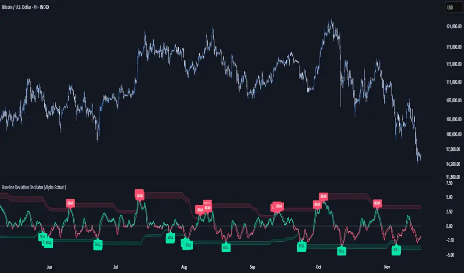
Baseline Deviation Oscillator [Alpha Extract]A sophisticated normalized oscillator system that measures price deviation from a customizable moving average baseline using ATR-based scaling and dynamic threshold adaptation. Utilizing advanced HL median filtering and multi-timeframe threshold calculations, this indicator delivers institutional-grade overbought/oversold detection with automatic zone adjustment based on recent oscillator extremes. The system's flexible baseline architecture supports six different moving average types while maintaining consistent ATR normalization for reliable signal generation across varying market volatility conditions.
🔶 Advanced Baseline Construction Framework
Implements flexible moving average architecture supporting EMA, RMA, SMA, WMA, HMA, and TEMA calculations with configurable source selection for optimal baseline customization. The system applies HL median filtering to the raw baseline for exceptional smoothing and outlier resistance, creating ultra-stable trend reference levels suitable for precise deviation measurement.
// Flexible Baseline MA System
ma(src, length, type) =>
if type == "EMA"
ta.ema(src, length)
else if type == "TEMA"
ema1 = ta.ema(src, length)
ema2 = ta.ema(ema1, length)
ema3 = ta.ema(ema2, length)
3 * ema1 - 3 * ema2 + ema3
// Baseline with HL Median Smoothing
Baseline_Raw = ma(src, MA_Length, MA_Type)
Baseline = hlMedian(Baseline_Raw, HL_Filter_Length)
🔶 ATR Normalization Engine
Features sophisticated ATR-based scaling methodology that normalizes price deviations relative to current volatility conditions, ensuring consistent oscillator readings across different market regimes. The system calculates ATR bands around the baseline and uses half the band width as the normalization factor for volatility-adjusted deviation measurement.
🔶 Dynamic Threshold Adaptation System
Implements intelligent threshold calculation using rolling window analysis of oscillator extremes with configurable smoothing and expansion parameters. The system identifies peak and trough levels over dynamic windows, applies EMA smoothing, and adds expansion factors to create adaptive overbought/oversold zones that adjust to changing market conditions.
1D
3D
1W
🔶 Multi-Source Configuration Architecture
Provides comprehensive source selection including Close, Open, HL2, HLC3, and OHLC4 options for baseline calculation, enabling traders to optimize oscillator behavior for specific trading styles. The flexible source system allows adaptation to different market characteristics while maintaining consistent ATR normalization methodology.
🔶 Signal Generation Framework
Generates bounce signals when oscillator crosses back through dynamic thresholds and zero-line crossover signals for trend confirmation. The system identifies both standard threshold bounces and extreme zone bounces with distinct alert conditions for comprehensive reversal and continuation pattern detection.
Bull_Bounce = ta.crossover(OSC, -Active_Lower) or
ta.crossover(OSC, -Active_Lower_Extreme)
Bear_Bounce = ta.crossunder(OSC, Active_Upper) or
ta.crossunder(OSC, Active_Upper_Extreme)
// Zero Line Signals
Zero_Cross_Up = ta.crossover(OSC, 0)
Zero_Cross_Down = ta.crossunder(OSC, 0)
🔶 Enhanced Visual Architecture
Provides color-coded oscillator line with bullish/bearish dynamic coloring, signal line overlay for trend confirmation, and optional cloud fills between oscillator and signal. The system includes gradient zone fills for overbought/oversold regions with configurable transparency and threshold level visualization with automatic label generation.
snapshot
🔶 HL Median Filter Integration
Features advanced high-low median filtering identical to DEMA Flow for exceptional baseline smoothing without lag introduction. The system constructs rolling windows of baseline values, performs median extraction for both odd and even window lengths, and eliminates outliers for ultra-clean deviation measurement baseline.
🔶 Comprehensive Alert System
Implements multi-tier alert framework covering bullish bounces from oversold zones, bearish bounces from overbought zones, and zero-line crossovers in both directions. The system provides real-time notifications for critical oscillator events with customizable message templates for automated trading integration.
🔶 Performance Optimization Framework
Utilizes efficient calculation methods with optimized array management for median filtering and minimal computational overhead for real-time oscillator updates. The system includes intelligent null value handling and automatic scale factor protection to prevent division errors during extreme market conditions.
🔶 Why Choose Baseline Deviation Oscillator ?
This indicator delivers sophisticated normalized oscillator analysis through flexible baseline architecture and dynamic threshold adaptation. Unlike traditional oscillators with fixed levels, the BDO automatically adjusts overbought/oversold zones based on recent oscillator behavior while maintaining consistent ATR normalization for reliable cross-market and cross-timeframe comparison. The system's combination of multiple MA type support, HL median filtering, and intelligent zone expansion makes it essential for traders seeking adaptive momentum analysis with reduced false signals and comprehensive reversal detection across cryptocurrency, forex, and equity markets.
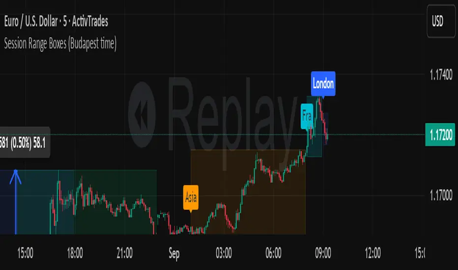
Session Range Boxes (Budapest time) GR V2.0Session Range Boxes (Budapest time)
This indicator draws intraday range boxes for the main Forex sessions based on Europe/Budapest time (CET/CEST).
Tracked sessions (Budapest time):
Asia: 01:00 – 08:00
Frankfurt (pre-London): 08:00 – 09:00
London: 09:00 – 18:00
New York: 14:30 – 23:00
For each session, the script:
Detects the session start and session end using the current chart timeframe and the Europe/Budapest time zone.
Tracks the high and low of price during the entire session.
Draws a box (rectangle) from session open to session close, covering the full price range between session high and low.
Optionally prints a small label above the first bar of each session (Asia, Fra, London, NY).
Color scheme:
Asia: soft orange box
Frankfurt: light aqua box
London: darker blue box
New York: light lime box
Use this tool to:
Quickly see which session created the high/low of the day,
Identify liquidity zones and session ranges that price may revisit,
Visually separate Asia, Frankfurt, London and New York volatility on intraday charts.
Optimized for intraday trading (Forex / indices), but it works on any symbol where session behavior matters.
Michael's Custom Watermark🔷 MICHAEL'S CUSTOM WATERMARK INDICATOR
━━━━━━━━━━━━━━━━━━━━━━━━━━━━━━━━━━━━━━━
📊 OVERVIEW
A comprehensive chart watermark overlay that displays essential fundamental and technical information for stocks in a clean, customizable table format. Perfect for traders who want quick access to key metrics without cluttering their charts.
━━━━━━━━━━━━━━━━━━━━━━━━━━━━━━━━━━━━━━━
✨ KEY FEATURES
📊 Fundamental Data Display — Shows Industry, Sector, Market Cap, and P/E Ratio
📅 Earnings Information — Displays next earnings date with countdown timer
📈 ATR Volatility Indicator — 14-day ATR with color-coded visual alerts (🔴🟡🟢)
🎨 Auto Theme Detection — Automatically adjusts text color based on chart background
⚙️ Fully Customizable — Position, colors, size, and displayed metrics all adjustable
🏢 GICS Sector Mapping — Heuristic-based sector classification aligned with industry standards
━━━━━━━━━━━━━━━━━━━━━━━━━━━━━━━━━━━━━━━
🎯 WHAT MAKES THIS INDICATOR UNIQUE?
Unlike basic watermarks, this indicator provides:
Real-time fundamental data integration
Smart theme-aware color adaptation for both light and dark charts
Configurable volatility alerts using ATR thresholds
Earnings countdown feature to never miss important dates
Optimized display that only shows relevant data for the current symbol type
━━━━━━━━━━━━━━━━━━━━━━━━━━━━━━━━━━━━━━━
📖 HOW TO USE
1. BASIC SETUP
Add the indicator to your chart. By default, it displays in the top-left corner with all features enabled.
2. POSITIONING
Vertical Location: Top, Middle, or Bottom
Horizontal Location: Left, Center, or Right
Vertical Offset: Fine-tune position with 0-50 pixel offset from top
3. CUSTOMIZATION OPTIONS
TEXT APPEARANCE:
Auto Text Color — Enable to automatically adapt text color to your chart theme
Manual Color — Set a fixed text color if auto-color is disabled
Text Size — Choose from Huge, Large, Normal, or Small
Theme Colors — Customize text color for light and dark backgrounds separately
DATA DISPLAY TOGGLES:
Show Industry & Sector — Display heuristic-based GICS-aligned sector and industry classification
Show Market Cap — View market capitalization in T/B/M format
Show P/E Ratio — Display Price-to-Earnings ratio (stocks only)
Show ATR (14-Day) — Display Average True Range with percentage and visual indicator
Show Next Earnings — Display upcoming earnings information
Show Earnings Countdown — Show days remaining until next earnings (requires earnings display)
4. ATR VOLATILITY ALERTS
Configure custom thresholds to monitor volatility:
Red Threshold — ATR percentage that triggers red alert 🔴 (default: 6%)
Yellow Threshold — ATR percentage that triggers yellow alert 🟡 (default: 3%)
Green — Shows automatically when ATR is below yellow threshold 🟢
━━━━━━━━━━━━━━━━━━━━━━━━━━━━━━━━━━━━━━━
📐 UNDERSTANDING THE DISPLAY
🏢 SECTOR & INDUSTRY
Shows the GICS sector classification followed by the specific industry. The indicator uses heuristic-based mapping to align TradingView sectors with standard GICS classifications. Note that this mapping is based on keyword detection and industry analysis, so while generally accurate, it may not perfectly match official GICS classifications in all cases.
💰 MARKET CAP
Displays market capitalization using standard abbreviations:
T = Trillion
B = Billion
M = Million
📊 P/E RATIO
Shows the trailing twelve-month Price-to-Earnings ratio. Only displayed for stocks when enabled. Shows "N/A" if data is unavailable.
📈 ATR (14-DAY)
Displays the 14-period Average True Range in both absolute value and percentage terms, with a color-coded indicator:
🔴 Red: High volatility (above red threshold)
🟡 Yellow: Moderate volatility (between yellow and red thresholds)
🟢 Green: Low volatility (below yellow threshold)
📅 EARNINGS
Shows earnings information in three formats:
"X days remaining" — When countdown is enabled and earnings date is known
"Upcoming" — When date is in the future but countdown is disabled
"Recently Reported" — When earnings just occurred
"N/A" — When no earnings data is available
━━━━━━━━━━━━━━━━━━━━━━━━━━━━━━━━━━━━━━━
⚙️ TECHNICAL DETAILS
SUPPORTED INSTRUMENTS:
Optimized for stocks with full fundamental data
Works with other instruments (crypto, forex, futures) but only displays applicable metrics
Automatically suppresses irrelevant data (e.g., P/E for non-stocks)
PERFORMANCE:
Lightweight overlay with minimal resource usage
Updates only on last bar for efficiency
No historical recalculation needed
COMPATIBILITY:
Pine Script v6
Works on all timeframes
Compatible with all chart types
Auto-adapts to theme changes
━━━━━━━━━━━━━━━━━━━━━━━━━━━━━━━━━━━━━━━
💡 TIPS & BEST PRACTICES
Enable Auto Text Color for seamless theme switching between light and dark modes
Adjust vertical offset to avoid overlap with price action in high-volatility periods
Use ATR thresholds appropriate to your trading style and asset class
Disable features you don't use to keep the watermark clean and focused
Position in corners to maximize chart viewing space
Use smaller text size for multi-panel layouts
━━━━━━━━━━━━━━━━━━━━━━━━━━━━━━━━━━━━━━━
🔧 TROUBLESHOOTING
"N/A" SHOWING FOR P/E RATIO:
This is normal for non-stock instruments
May occur for stocks with negative earnings
Check if fundamental data is available for the symbol
EARNINGS SHOWING "N/A":
Earnings data may not be available for all stocks
Check TradingView's data coverage for your symbol
TEXT COLOR NOT VISIBLE:
Enable Auto Text Color feature
Manually set text color to contrast with your chart background
Adjust custom light/dark text colors in settings
━━━━━━━━━━━━━━━━━━━━━━━━━━━━━━━━━━━━━━━
⚠️ DISCLAIMER
This indicator is for informational purposes only. The fundamental data displayed is sourced from TradingView's data providers. Always verify critical information before making trading decisions. Past performance is not indicative of future results.
━━━━━━━━━━━━━━━━━━━━━━━━━━━━━━━━━━━━━━━
If you find this indicator helpful, please give it a boost 🚀 and share your feedback in the comments!
Version: 1.0
Pine Script Version: v6
Created by: Michael
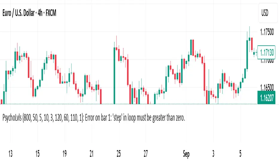
Psychological Levels (Zones + Alerts) - StableThis technical indicator plot support and resistance levels based on the psychological numbers
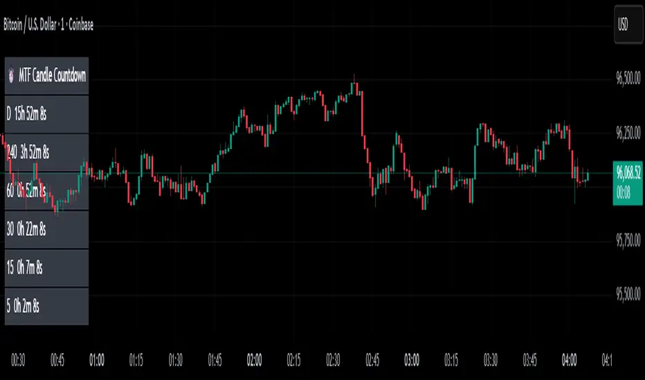
MTF Candle Countdown — HUD V1 (By Price-Action-Art)
MTF Candle Countdown — HUD V1 (By Price-Action-Art)
A clean, lightweight HUD that shows you exactly how much time is left in multiple higher-timeframe candles — all in one place.
This tool is designed for traders who rely on multi-timeframe precision.
Instead of constantly switching charts or checking timers, the HUD gives you a real-time countdown for up to six timeframes (Daily, 4H, 1H, 30m, 15m, 5m by default).
You can fully customize the timeframes, text size, and HUD position on your chart.
Perfect for:
Intraday and scalping timing
Swing traders waiting for HTF candle closes
ICT / SMC structure-based traders
Anyone who needs exact candle close timing without distractions
Features:
Real-time multi-timeframe candle countdown
Fully adjustable HUD placement (all corners)
Customizable timeframes and text size
Clean, minimal, and non-intrusive design
Updates only on the last bar for performance efficiency
Optional border for a sharper HUD look
Whether you’re waiting for a Daily close to confirm structure or timing your entries around 5m/15m candles, this HUD keeps everything visible and precise at a glance.
If you find this tool helpful, feel free to like, comment, and follow — it motivates me to keep releasing more tools for the community.
Rons Custom WatermarkRon's Custom Watermark (RCW)
This is a lightweight, all-in-one watermark indicator that displays essential fundamental and technical data directly on your chart. It's designed to give you a quick, at-a-glance overview of any asset without cluttering your screen.
Features
The watermark displays the following information in a clean table:
* Company Info: Full Name & Market Cap (e.g., "AST SpaceMobile, Inc. (18.85B)")
* Symbol & Timeframe: Ticker and current chart period (e.g., "ASTS, 1D")
* Sector & Industry: The asset's classification.
* Technical Status (MA): Shows if the price is Above or Below the SMA (with a 🟢/🔴 emoji).
* Technical Status (EMA): Shows if the price is Above or Below the EMA (with a 🟢/🔴 emoji).
* Earnings: A countdown showing "X days remaining" until the next earnings report.
* (Optional) Volatility: The 14-day ATR value and its percentage of the current price.

Weekly Fibonacci Pivot Signals (4H) - S1/R1 & S3/R3 rulesThis Indicator used weekly price range to calculate the pivot R1,R3,S1 and S3 ,when price crossed and closed below R3 in 4H timeframe the indicator gives sell signal, when the price crossed and close above the S3 the indicator gives buy signal. This indicator can give approximately 50% win Rate .

Market Extreme Zones IndexThe Market Extreme Zones Index is a new mean reversion (valuation) tool focused on catching long term oversold/overbought zones. Combining an enhanced RSI with a smoothed Z-score this indicator allows traders to find oppurtunities during highly oversold/overbought zones.
I will separate the explanation into the following parts:
1. How does it work?
2. Methodologies & Concepts
3. Use cases
How does it work?
The indicator attempts to catch highly unprobable events in either direction to capture reversal points over the long term. This is done by calculating the Z-Score of an enhanced RSI.
First we need to calculate the Enhanced RSI:
For this we need to calculate 2 additional lengths:
Length1 = user defined length
Length2 = Length1/2
Length3 = √Length
Now we need to calculate 3 different RSIs:
1st RSI => uses classic user defined source and classic user defined length.
2nd RSI => uses classic user defined source and Length 2.
3rd RSI => uses RSI 2 as source and Length 2
Now calculate the divergence:
RSI_base => 2nd RSI * 3 - 1st RSI - 3rd RSI
After this we need to calculate the median of the RSI_base over √Length and make a divergence of these 2:
RSI => RSI_base*2 - median
All that remains now is the Z-score calculations:
We need:
Average RSI value
Standard Deviation = a measure of how dispersed or spread out a set of data values are from their average
Z-score = (Current Value - Average Value) / Standard Deviation
After this we just smooth the Z-score with a Weighted Moving average with √Length
Methodology & Concepts
Mean Reversion Methodology:
The methodology behind mean reversion is the theory that asset prices will eventually return to their long-term average after deviating significantly, driven by the belief that extreme moves are temporary.
Z-Score Methodology:
A Z-score, or standard score, is a statistical measure that indicates how many standard deviations a data point is from the mean of a dataset. A positive z-score means the value is above the mean, a negative score means it's below, and a score of zero means the value is equal to the mean.
You might already be able to see where I am going with this:
Z-Score could be used for the extreme moves to capture reversal points.
By applying it to the RSI rather than the Price, we get a more accurate measurement that allow us to get a banger indicator.
Use Cases
Capturing reversal points
Trend Direction
- while the main use it for mean reversion, the values can indicate whether we are in an uptrend or a downtrend.
Advantages:
Visualization:
The indicator has many plots to ensure users can easily see what the indicator signals, such as highlighting extreme conditions with background colors.
Versatility:
This indicator works across multiple assets, including the S&P500 and more, so it is not only for crypto.
Final note:
No indicator alone is perfect.
Backtests are not indicative of future performance.
Hope you enjoy Gs!
Good luck!

Checklist (D1 / H4 / M15/30 BoS / VP / Fibo / S/R) This is a simple, visual checklist indicator that allows you to quickly assess how many of your strategy conditions are met, without affecting the chart itself. It is ideal for multi-timeframe strategies and point-by-point setup monitoring.

Volatility-Targeted Momentum Portfolio [BackQuant]Volatility-Targeted Momentum Portfolio
A complete momentum portfolio engine that ranks assets, targets a user-defined volatility, builds long, short, or delta-neutral books, and reports performance with metrics, attribution, Monte Carlo scenarios, allocation pie, and efficiency scatter plots. This description explains the theory and the mechanics so you can configure, validate, and deploy it with intent.
Table of contents
What the script does at a glance
Momentum, what it is, how to know if it is present
Volatility targeting, why and how it is done here
Portfolio construction modes: Long Only, Short Only, Delta Neutral
Regime filter and when the strategy goes to cash
Transaction cost modelling in this script
Backtest metrics and definitions
Performance attribution chart
Monte Carlo simulation
Scatter plot analysis modes
Asset allocation pie chart
Inputs, presets, and deployment checklist
Suggested workflow
1) What the script does at a glance
Pulls a list of up to 15 tickers, computes a simple momentum score on each over a configurable lookback, then volatility-scales their bar-to-bar return stream to a target annualized volatility.
Ranks assets by raw momentum, selects the top 3 and bottom 3, builds positions according to the chosen mode, and gates exposure with a fast regime filter.
Accumulates a portfolio equity curve with risk and performance metrics, optional benchmark buy-and-hold for comparison, and a full alert suite.
Adds visual diagnostics: performance attribution bars, Monte Carlo forward paths, an allocation pie, and scatter plots for risk-return and factor views.
2) Momentum: definition, detection, and validation
Momentum is the tendency of assets that have performed well to continue to perform well, and of underperformers to continue underperforming, over a specific horizon. You operationalize it by selecting a horizon, defining a signal, ranking assets, and trading the leaders versus laggards subject to risk constraints.
Signal choices . Common signals include cumulative return over a lookback window, regression slope on log-price, or normalized rate-of-change. This script uses cumulative return over lookback bars for ranking (variable cr = price/price - 1). It keeps the ranking simple and lets volatility targeting handle risk normalization.
How to know momentum is present .
Leaders and laggards persist across adjacent windows rather than flipping every bar.
Spread between average momentum of leaders and laggards is materially positive in sample.
Cross-sectional dispersion is non-trivial. If everything is flat or highly correlated with no separation, momentum selection will be weak.
Your validation should include a diagnostic that measures whether returns are explained by a momentum regression on the timeseries.
Recommended diagnostic tool . Before running any momentum portfolio, verify that a timeseries exhibits stable directional drift. Use this indicator as a pre-check: It fits a regression to price, exposes slope and goodness-of-fit style context, and helps confirm if there is usable momentum before you force a ranking into a flat regime.
3) Volatility targeting: purpose and implementation here
Purpose . Volatility targeting seeks a more stable risk footprint. High-vol assets get sized down, low-vol assets get sized up, so each contributes more evenly to total risk.
Computation in this script (per asset, rolling):
Return series ret = log(price/price ).
Annualized volatility estimate vol = stdev(ret, lookback) * sqrt(tradingdays).
Leverage multiplier volMult = clamp(targetVol / vol, 0.1, 5.0).
This caps sizing so extremely low-vol assets don’t explode weight and extremely high-vol assets don’t go to zero.
Scaled return stream sr = ret * volMult. This is the per-bar, risk-adjusted building block used in the portfolio combinations.
Interpretation . You are not levering your account on the exchange, you are rescaling the contribution each asset’s daily move has on the modeled equity. In live trading you would reflect this with position sizing or notional exposure.
4) Portfolio construction modes
Cross-sectional ranking . Assets are sorted by cr over the chosen lookback. Top and bottom indices are extracted without ties.
Long Only . Averages the volatility-scaled returns of the top 3 assets: avgRet = mean(sr_top1, sr_top2, sr_top3). Position table shows per-asset leverages and weights proportional to their current volMult.
Short Only . Averages the negative of the volatility-scaled returns of the bottom 3: avgRet = mean(-sr_bot1, -sr_bot2, -sr_bot3). Position table shows short legs.
Delta Neutral . Long the top 3 and short the bottom 3 in equal book sizes. Each side is sized to 50 percent notional internally, with weights within each side proportional to volMult. The return stream mixes the two sides: avgRet = mean(sr_top1,sr_top2,sr_top3, -sr_bot1,-sr_bot2,-sr_bot3).
Notes .
The selection metric is raw momentum, the execution stream is volatility-scaled returns. This separation is deliberate. It avoids letting volatility dominate ranking while still enforcing risk parity at the return contribution stage.
If everything rallies together and dispersion collapses, Long Only may behave like a single beta. Delta Neutral is designed to extract cross-sectional momentum with low net beta.
5) Regime filter
A fast EMA(12) vs EMA(21) filter gates exposure.
Long Only active when EMA12 > EMA21. Otherwise the book is set to cash.
Short Only active when EMA12 < EMA21. Otherwise cash.
Delta Neutral is always active.
This prevents taking long momentum entries during obvious local downtrends and vice versa for shorts. When the filter is false, equity is held flat for that bar.
6) Transaction cost modelling
There are two cost touchpoints in the script.
Per-bar drag . When the regime filter is active, the per-bar return is reduced by fee_rate * avgRet inside netRet = avgRet - (fee_rate * avgRet). This models proportional friction relative to traded impact on that bar.
Turnover-linked fee . The script tracks changes in membership of the top and bottom baskets (top1..top3, bot1..bot3). The intent is to charge fees when composition changes. The template counts changes and scales a fee by change count divided by 6 for the six slots.
Use case: increase fee_rate to reflect taker fees and slippage if you rebalance every bar or trade illiquid assets. Reduce it if you rebalance less often or use maker orders.
Practical advice .
If you rebalance daily, start with 5–20 bps round-trip per switch on liquid futures and adjust per venue.
For crypto perp microcaps, stress higher cost assumptions and add slippage buffers.
If you only rotate on lookback boundaries or at signals, use alert-driven rebalances and lower per-bar drag.
7) Backtest metrics and definitions
The script computes a standard set of portfolio statistics once the start date is reached.
Net Profit percent over the full test.
Max Drawdown percent, tracked from running peaks.
Annualized Mean and Stdev using the chosen trading day count.
Variance is the square of annualized stdev.
Sharpe uses daily mean adjusted by risk-free rate and annualized.
Sortino uses downside stdev only.
Omega ratio of sum of gains to sum of losses.
Gain-to-Pain total gains divided by total losses absolute.
CAGR compounded annual growth from start date to now.
Alpha, Beta versus a user-selected benchmark. Beta from covariance of daily returns, Alpha from CAPM.
Skewness of daily returns.
VaR 95 linear-interpolated 5th percentile of daily returns.
CVaR average of the worst 5 percent of daily returns.
Benchmark Buy-and-Hold equity path for comparison.
8) Performance attribution
Cumulative contribution per asset, adjusted for whether it was held long or short and for its volatility multiplier, aggregated across the backtest. You can filter to winners only or show both sides. The panel is sorted by contribution and includes percent labels.
9) Monte Carlo simulation
The panel draws forward equity paths from either a Normal model parameterized by recent mean and stdev, or non-parametric bootstrap of recent daily returns. You control the sample length, number of simulations, forecast horizon, visibility of individual paths, confidence bands, and a reproducible seed.
Normal uses Box-Muller with your seed. Good for quick, smooth envelopes.
Bootstrap resamples realized returns, preserving fat tails and volatility clustering better than a Gaussian assumption.
Bands show 10th, 25th, 75th, 90th percentiles and the path mean.
10) Scatter plot analysis
Four point-cloud modes, each plotting all assets and a star for the current portfolio position, with quadrant guides and labels.
Risk-Return Efficiency . X is risk proxy from leverage, Y is expected return from annualized momentum. The star shows the current book’s composite.
Momentum vs Volatility . Visualizes whether leaders are also high vol, a cue for turnover and cost expectations.
Beta vs Alpha . X is a beta proxy, Y is risk-adjusted excess return proxy. Useful to see if leaders are just beta.
Leverage vs Momentum . X is volMult, Y is momentum. Shows how volatility targeting is redistributing risk.
11) Asset allocation pie chart
Builds a wheel of current allocations.
Long Only, weights are proportional to each long asset’s current volMult and sum to 100 percent.
Short Only, weights show the short book as positive slices that sum to 100 percent.
Delta Neutral, 50 percent long and 50 percent short books, each side leverage-proportional.
Labels can show asset, percent, and current leverage.
12) Inputs and quick presets
Core
Portfolio Strategy . Long Only, Short Only, Delta Neutral.
Initial Capital . For equity scaling in the panel.
Trading Days/Year . 252 for stocks, 365 for crypto.
Target Volatility . Annualized, drives volMult.
Transaction Fees . Per-bar drag and composition change penalty, see the modelling notes above.
Momentum Lookback . Ranking horizon. Shorter is more reactive, longer is steadier.
Start Date . Ensure every symbol has data back to this date to avoid bias.
Benchmark . Used for alpha, beta, and B&H line.
Diagnostics
Metrics, Equity, B&H, Curve labels, Daily return line, Rolling drawdown fill.
Attribution panel. Toggle winners only to focus on what matters.
Monte Carlo mode with Normal or Bootstrap and confidence bands.
Scatter plot type and styling, labels, and portfolio star.
Pie chart and labels for current allocation.
Presets
Crypto Daily, Long Only . Lookback 25, Target Vol 50 percent, Fees 10 bps, Regime filter on, Metrics and Drawdown on. Monte Carlo Bootstrap with Recent 200 bars for bands.
Crypto Daily, Delta Neutral . Lookback 25, Target Vol 50 percent, Fees 15–25 bps, Regime filter always active for this mode. Use Scatter Risk-Return to monitor efficiency and keep the star near upper left quadrants without drifting rightward.
Equities Daily, Long Only . Lookback 60–120, Target Vol 15–20 percent, Fees 5–10 bps, Regime filter on. Use Benchmark SPX and watch Alpha and Beta to keep the book from becoming index beta.
13) Suggested workflow
Universe sanity check . Pick liquid tickers with stable data. Thin assets distort vol estimates and fees.
Check momentum existence . Run on your timeframe. If slope and fit are weak, widen lookback or avoid that asset or timeframe.
Set risk budget . Choose a target volatility that matches your drawdown tolerance. Higher target increases turnover and cost sensitivity.
Pick mode . Long Only for bull regimes, Short Only for sustained downtrends, Delta Neutral for cross-sectional harvesting when index direction is unclear.
Tune lookback . If leaders rotate too often, lengthen it. If entries lag, shorten it.
Validate cost assumptions . Increase fee_rate and stress Monte Carlo. If the edge vanishes with modest friction, refine selection or lengthen rebalance cadence.
Run attribution . Confirm the strategy’s winners align with intuition and not one unstable outlier.
Use alerts . Enable position change, drawdown, volatility breach, regime, momentum shift, and crash alerts to supervise live runs.
Important implementation details mapped to code
Momentum measure . cr = price / price - 1 per symbol for ranking. Simplicity helps avoid overfitting.
Volatility targeting . vol = stdev(log returns, lookback) * sqrt(tradingdays), volMult = clamp(targetVol / vol, 0.1, 5), sr = ret * volMult.
Selection . Extract indices for top1..top3 and bot1..bot3. The arrays rets, scRets, lev_vals, and ticks_arr track momentum, scaled returns, leverage multipliers, and display tickers respectively.
Regime filter . EMA12 vs EMA21 switch determines if the strategy takes risk for Long or Short modes. Delta Neutral ignores the gate.
Equity update . Equity multiplies by 1 + netRet only when the regime was active in the prior bar. Buy-and-hold benchmark is computed separately for comparison.
Tables . Position tables show current top or bottom assets with leverage and weights. Metric table prints all risk and performance figures.
Visualization panels . Attribution, Monte Carlo, scatter, and pie use the last bars to draw overlays that update as the backtest proceeds.
Final notes
Momentum is a portfolio effect. The edge comes from cross-sectional dispersion, adequate risk normalization, and disciplined turnover control, not from a single best asset call.
Volatility targeting stabilizes path but does not fix selection. Use the momentum regression link above to confirm structure exists before you size into it.
Always test higher lag costs and slippage, then recheck metrics, attribution, and Monte Carlo envelopes. If the edge persists under stress, you have something robust.
