ค้นหาในสคริปต์สำหรับ "trend"

Pivot Reversal Strategy - FIGS & DATES 2.0Simple Pivot Reversal Strategy with some adding settings.
Date Range: To test over specific market conditions.
Initial Capitol: $10K - This is a more realistic representation of funds used this strategy (for me anyway). The default of $100K can give different results (usually better) than when using a smaller balance.
Order Size: 100% Equity - These trend following strategies typically used this way, going all in each direction.
Commission: .075% - It's always disheartening to think you've found a ridiculously good setting, and then realize you forgot to add the commission.
All of these settings can be changed, but it's easier for me (and more fool proof) to have them set as default.

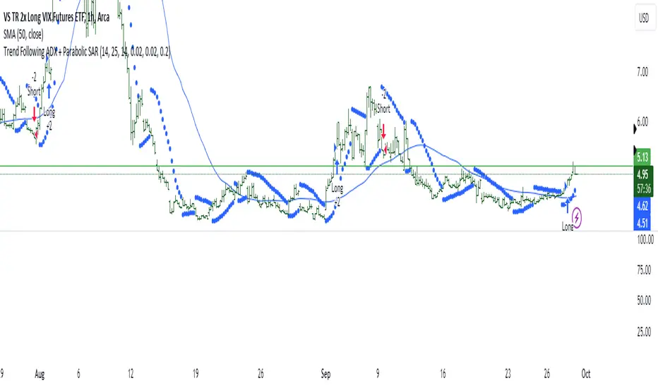
Trend Following ADX + Parabolic SAR### Strategy Description: Trend Following using **ADX** and **Parabolic SAR**
This strategy is designed to follow market trends using two popular indicators: **Average Directional Index (ADX)** and **Parabolic SAR**. The strategy attempts to enter trades when the market shows a strong trend (using ADX) and confirms the trend direction using the Parabolic SAR. Here's a breakdown:
### Key Indicators:
1. **ADX (Average Directional Index)**:
- **Purpose**: ADX measures the strength of a trend, regardless of direction.
- **Usage**: The strategy uses ADX to confirm that the market is trending. When ADX is above a certain threshold (e.g., 25), it indicates a strong trend.
- **Directional Indicators**:
- **DI+ (Directional Indicator Plus)**: Indicates upward movement strength.
- **DI- (Directional Indicator Minus)**: Indicates downward movement strength.
2. **Parabolic SAR**:
- **Purpose**: Parabolic SAR is a trend-following indicator used to identify potential reversals in the price direction.
- **Usage**: It provides specific price points above or below which the strategy confirms buy or sell signals.
### Strategy Logic:
#### **Entry Conditions**:
1. **Long Position** (Buy):
- **ADX** is above the threshold (default: 25), indicating a strong trend.
- **DI+ > DI-**, indicating the upward trend is stronger than the downward.
- The price is above the **Parabolic SAR** level, confirming the upward trend.
2. **Short Position** (Sell):
- **ADX** is above the threshold (default: 25), indicating a strong trend.
- **DI- > DI+**, indicating the downward trend is stronger than the upward.
- The price is below the **Parabolic SAR** level, confirming the downward trend.
#### **Exit Conditions**:
- Positions are closed when an opposite signal is detected.
- For example, if a long position is open and the conditions for a short position are met, the long position is closed, and a short position is opened.
### Parameters:
1. **ADX Period**: Defines the length of the period for the ADX calculation (default: 14).
2. **ADX Threshold**: The minimum value of ADX to confirm a strong trend (default: 25).
3. **Parabolic SAR Start**: The initial step for the SAR (default: 0.02).
4. **Parabolic SAR Increment**: The step increment for SAR (default: 0.02).
5. **Parabolic SAR Max**: The maximum step for SAR (default: 0.2).
### Example Trade Flow:
#### **Long Trade**:
1. ADX > 25, confirming a strong trend.
2. DI+ > DI-, indicating the market is trending upward.
3. The price is above the Parabolic SAR, confirming the upward direction.
4. **Action**: Enter a long (buy) position.
5. Exit the long position when a short signal is triggered (i.e., DI- > DI+, price below Parabolic SAR).
#### **Short Trade**:
1. ADX > 25, confirming a strong trend.
2. DI- > DI+, indicating the market is trending downward.
3. The price is below the Parabolic SAR, confirming the downward direction.
4. **Action**: Enter a short (sell) position.
5. Exit the short position when a long signal is triggered (i.e., DI+ > DI-, price above Parabolic SAR).
### Strengths of the Strategy:
- **Trend-Following**: It performs well in markets with strong trends, whether upward or downward.
- **Dual Confirmation**: The combination of ADX and Parabolic SAR reduces false signals by ensuring both trend strength and direction are considered before entering a trade.
### Weaknesses:
- **Range-Bound Markets**: This strategy may perform poorly in choppy, non-trending markets because both ADX and SAR are trend-following indicators.
- **Lagging Nature**: Since both ADX and SAR are lagging indicators, the strategy may enter trades after the trend has already started, potentially missing early profits.
### Customization:
- **ADX Threshold**: You can increase the threshold if you only want to trade in very strong trends, or lower it to capture more moderate trends.
- **SAR Parameters**: Adjusting the SAR `start`, `increment`, and `max` values will make the Parabolic SAR more or less sensitive to price changes.
### Summary:
This strategy combines the ADX and Parabolic SAR to take advantage of strong market trends. By confirming both trend strength (ADX) and trend direction (Parabolic SAR), it aims to enter high-probability trades in trending markets while minimizing false signals. However, it may struggle in sideways or non-trending markets.
For Educational purposes only !!!
Dow Theory based Strategy (Markttechnik)What makes this script unique?
calculates two trends at the same time: a big one for the overall strong trend - and a small one to trigger a trade after a small correction within the big trend
only if both trends (the small and the big trend) are in an uptrend, a buy signal is created: this prevents a buy signal from being generated in a falling market just because an upward movement begins in a small trend
the exit strategy can be configured very flexibly and individually: use the last low as stop loss and automatically switch to a trialing stop loss as soon as the take profit is reached (instead of finishing the trade)
the take profit strategy can also be configured - e.g. use the last high, a fixed percentage or a combination of it
plots each trade in detail on the chart - e.g. inner candles or the exact progression of the stop loss over the entire duration of the trade to allow you to analyze each trade precisely
What does the script do and how?
In this strategy an intact upward trend is characterized by higher highs and lower lows only if the big trend and the small trend are in an upward trend at the same time.
The following describes how the script calculates a buy signal. Every step is drawn to the chart immediately - see example chart above:
1. the stock rises in the big trend - i.e. in a longer time frame
2. a correction takes place (the share price falls) - but does not create a new low
3. the stock rises again in the big trend and creates a new high
From now on, the big trend is in an intact upward trend (until it falls below its last low).
This is drawn to the chart as 3 bold green zigzag lines.
But we do not buy right now! Instead, we want to wait for a correction in the big trend and for the start of a small upward trend.
4. a correction takes place (not below the low from 2.)
Now, the script also starts to calculate the small trend:
5. the stock rises in the small trend - i.e. in a shorter time frame
6. a small correction takes place (not below the low from 4.)
7. the stock rises above the high from 5.: a new high in the shorter time frame
Now, both trends are in an intact upward trend.
A buy signal is created and both the minor and major trend are colored green on the chart.
Now, the trade is active and:
the stop loss is calculated and drawn for each candle
the take profit is calculated and drawn to the chart
as soon as the price reaches the take profit or the stop loss, the trade is closed
Features and functionalities
Uptrend : An intact upward trend is characterized by higher highs and lower lows. Uptrends are shown in green on the chart.
The beginning of an uptrend is numbered 1, each subsequent high is numbered 2, and each low is numbered 3.
Downtrend: An intact downtrend is characterized by lower highs and lower lows. Downtrends are displayed in red on the chart.
Note that our indicator does not show the numbering of the points of the downtrend.
Trendless phases: If there is no intact trend, we are in a trendless phase. Trendless phases are shown in blue on the chart.
This occurs after an uptrend, when a lower low or a lower high is formed. Or after a downtrend, when a higher low or a higher high is formed.
Buy signals
A buy signal is generated as soon as a new upward trend has been formed or a new high has been established in an intact upward trend.
But even before a buy signal is generated, this strategy anticipates a possible emerging trend and draws the next possible trading opportunity to the chart.
In addition to the (not yet reached) buy price, the risk-reward ratio, the StopLoss and the TakeProfit price is shown.
With this information, you can already enter a StopBuy order, which is thus triggered directly with the then created buy signal.
You can configure, if a buy signal shall be created while the big trend is an uptrend, a downtrend and/or trendless.
Exit strategy
With this strategy, you have multiple possibilities to close your position. All of them can be configured within the settings. In general, you can combine a take profit strategy with a stop loss strategy.
The take profit price will be calculated once for each trade. It will be drawn to the chart for active trade.
Depending on your configuration, this can be the last high (which is often a resistance level), a fixed percentage added to the buy price or the maximum of both.
You can also configure that a trailing stop loss is used as soon as the take profit price is reached once.
The stop loss gets recalculated with each candle and is displayed and plotted for each active and finished trade. With this, you can easily check how the stop loss changed during your trades.
The stop loss can be configured flexibly:
Use the classic "trailing stop loss" that follows the price from below.
Set the stop loss to the last low and tighten it every time the small trend marks a new local low.
Confiure that the stop loss is tightened as soon as the break even is reached. Nothing is more annoying than a trade turning from a win to a loss.
Ignore inside candles (see description below) and relax the stop loss to use the outside candle for its calculation.
Inner candles
Inner candles are created when the candle body is within the maximum values of a previous candle (the outer candle). There can be any number of consecutive inner candles. As soon as you have activated the "Check inner candles" setting, all consecutive inner candles will be highlighted in yellow on the chart.
Prices during an inner candle scenario might be irrelevant for trading and can be interpreted as fluctuations within the outside candle. For this reason, the trailing stop loss should not be aligned with inner candles. Therefore, as soon as an inner candle occurs, the stop loss is reset and the low at the time of the outside candle is used as the calculation for the trailing stop loss. This will all be plotted for you on the chart.
Display of the trades:
All active and closed trades of the last 5 years are displayed in the chart with buy signal, sell, stop loss history, inside candles and statistics.
Backtesting:
The strategy can be simulated for each stock over the period of the last 5 years. Each individual trade is recorded and can be traced and analyzed in the chart including stop loss history. Detailed evaluations and statistics are available to evaluate the performance of the strategy.
Additional Statistics
This strategy immediately displays a statistic table to the chart area giving you an overview of its performance over the last years for the given chart.
This includes:
The total win/loss in $ and %
The win/loss per year in %
The active investment time in days and % (e.g. invested 10 of 100 trading days -> 10%)
The total win/loss in %, extrapolated to 100% equity usage: Only with this value can strategies really be compared. Because you are not invested between the trades and could invest in other stocks during this time. This value indicates how much profit you would have made if you had been invested 100% of the time - or to put it another way - if you had been invested 100% of the time in stocks with exactly the same performance. Let's say you had only one trade in the last 5 years that lasted, say, only one month and made 5% profit. This would be significantly better than a strategy with which you were invested for, say, 5 years and made 10% profit.
The total profit/loss per year in %, extrapolated to 100% equity usage
Notifications (alerts):
Get alerted before a new buy signal emerges to create an order if necessary and not miss a trade. You can also be notified when the stop loss needs to be adjusted. The notification can be done in different ways, e.g. by Mail, PopUp or App-Notification. This saves them the annoying, time-consuming and error-prone "click through" all the charts.
Settings: Display Settings
With these settings, you have the possibility to:
Show the small or the big trend as a background color
Configure if the numbers (1-2-3-2-3) shall be shown at all or only for the small, the big trend or both
Settings: Trend calculation - fine tuning
Drawing trend lines on a chart is not an exact science. Some highs and lows are not very clear or significant. And so it will always happen that 2 different people would draw different trendlines for the same chart. Unfortunately, there is no exact "right" or "wrong" here.
With the options under "Trend Calculation - Fine Tuning" you have the possibility to influence the drawing in of trends and to adapt it to your personal taste.
Small Trend, Big Trend : With these settings you can influence how significant a high or low has to be to recognize them as an independent high or low. The larger the values, the more significant a high or low must be to be recognized as such.
High and low recognition : With this setting you can influence when two adjacent, almost identical highs or lows should be recognized as independent highs or lows. The higher the value, the more different "similar" highs or lows must be in order to be recognized as such.
Which default settings were selected and why
Show Trades: true - its often useful to see all recent trades in the chart
Time Frame: 1 day - most common time frame (except for day traders)
Take Profit: combined 10% - the last high is taken as take profit because the trend often changes there, but only if there is at least 10% profit to ensure we do not risk money for a tiny profit
Stop Loss: combined - the last low is used as stop loss because the trend would break there and switch to a trailing stop loss as soon as our take profit is reached to let our profits run without risking them anymore
Stop Loss distance: 3% - we are giving the price 3% air (below the last low) to avoid being stopped out due to a short price drop
Trailing Stop Loss: 2% - we have to give the stop loss some room to avoid being stopped out prematurely; this is a value that is well balanced between a certain downside distance and the profit-taking ratio
Set Stop Loss to break even: true, 2% - once we reached the break even, it is a common practice to not risk our money anymore, the value is set to the same value as the trailing stop loss
Trade Filter: Uptrend - we only start trades if the big trend is an uptrend in the expectation that it will continue after a small correction
Display settings: those will not influence the trades, feel free to change them to your needs
Trend calculation - Fine Tuning: 1/1,5/0,05; influences the internal calculation for highs and lows and how significant they need to be to be considered a new high or low; the default values will provide you nicely calculated trends in the daily time frame; if there are too many or too few lows and highs according to your taste, feel free to play around and immediately see the result drawn to the chart; read the manual for a detailed description of this values
Note that you can (and should) configure the general trading properties like your initial capital, order size, slippage and commission.

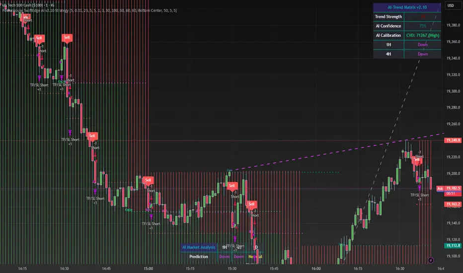
PowerHouse SwiftEdge AI v2.10 StrategyOverview
The PowerHouse SwiftEdge AI v2.10 Strategy is a sophisticated trading system designed to identify high-probability trade setups in forex, stocks, and cryptocurrencies. By combining multi-timeframe trend analysis, momentum signals, volume confirmation, and smart money concepts (Change of Character and Break of Structure ), this strategy offers traders a robust tool to capitalize on market trends while minimizing false signals. The strategy’s unique “AI” component analyzes trends across multiple timeframes to provide a clear, actionable dashboard, making it accessible for both novice and experienced traders. The strategy is fully customizable, allowing users to tailor its filters to their trading style.
What It Does
This strategy generates Buy and Sell signals based on a confluence of technical indicators and smart money concepts. It uses:
Multi-Timeframe Trend Analysis: Confirms the market’s direction by analyzing trends on the 1-hour (60M), 4-hour (240M), and daily (D) timeframes.
Momentum Filter: Ensures trades align with strong price movements to avoid choppy markets.
Volume Filter: Validates signals with above-average volume to confirm market participation.
Breakout Filter: Requires price to break key levels for added confirmation.
Smart Money Signals (CHoCH/BOS): Identifies reversals (CHoCH) and trend continuations (BOS) based on pivot points.
AI Trend Dashboard: Summarizes trend strength, confidence, and predictions across timeframes, helping traders make informed decisions without needing to analyze complex data manually.
The strategy also plots dynamic support and resistance trendlines, take-profit (TP) levels, and “Get Ready” signals to alert users of potential setups before they fully develop. Trades are executed with predefined take-profit and stop-loss levels for disciplined risk management.
How It Works
The strategy integrates multiple components to create a cohesive trading system:
Multi-Timeframe Trend Analysis:
The strategy evaluates trends on three timeframes (1H, 4H, Daily) using Exponential Moving Averages (EMA) and Volume-Weighted Average Price (VWAP). A trend is considered bullish if the price is above both the EMA and VWAP, bearish if below, or neutral otherwise.
Signals are only generated when the trend on the user-selected higher timeframe aligns with the trade direction (e.g., Buy signals require a bullish higher timeframe trend). This reduces noise and ensures trades follow the broader market context.
Momentum Filter:
Measures the percentage price change between consecutive bars and compares it to a volatility-adjusted threshold (based on the Average True Range ). This ensures trades are taken only during significant price movements, filtering out low-momentum conditions.
Volume Filter (Optional):
Checks if the current volume exceeds a long-term average and shows positive short-term volume change. This confirms strong market participation, reducing the risk of false breakouts.
Breakout Filter (Optional):
Requires the price to break above (for Buy) or below (for Sell) recent highs/lows, ensuring the signal aligns with a structural shift in the market.
Smart Money Concepts (CHoCH/BOS):
Change of Character (CHoCH): Detects potential reversals when the price crosses under a recent pivot high (for Sell) or over a recent pivot low (for Buy) with a bearish or bullish candle, respectively.
Break of Structure (BOS): Confirms trend continuations when the price breaks below a recent pivot low (for Sell) or above a recent pivot high (for Buy) with strong momentum.
These signals are plotted as horizontal lines with labels, making it easy to visualize key levels.
AI Trend Dashboard:
Combines trend direction, momentum, and volatility (ATR) across timeframes to calculate a trend score. Scores above 0.5 indicate an “Up” trend, below -0.5 indicate a “Down” trend, and otherwise “Neutral.”
Displays a table summarizing trend strength (as a percentage), AI confidence (based on trend alignment), and Cumulative Volume Delta (CVD) for market context.
A second table (optional) shows trend predictions for 1H, 4H, and Daily timeframes, helping traders anticipate future market direction.
Dynamic Trendlines:
Plots support and resistance lines based on recent swing lows and highs within user-defined periods (shortTrendPeriod, longTrendPeriod). These lines adapt to market conditions and are colored based on trend strength.
Why This Combination?
The PowerHouse SwiftEdge AI v2.10 Strategy is original because it seamlessly integrates traditional technical analysis (EMA, VWAP, ATR, volume) with smart money concepts (CHoCH, BOS) and a proprietary AI-driven trend analysis. Unlike standalone indicators, this strategy:
Reduces False Signals: By requiring confluence across trend, momentum, volume, and breakout filters, it minimizes trades in choppy or low-conviction markets.
Adapts to Market Context: The ATR-based momentum threshold adjusts dynamically to volatility, ensuring signals remain relevant in both trending and ranging markets.
Simplifies Decision-Making: The AI dashboard distills complex multi-timeframe data into a user-friendly table, eliminating the need for manual analysis.
Leverages Smart Money: CHoCH and BOS signals capture institutional price action patterns, giving traders an edge in identifying reversals and continuations.
The combination of these components creates a balanced system that aligns short-term trade entries with longer-term market trends, offering a unique blend of precision, adaptability, and clarity.
How to Use
Add to Chart:
Apply the strategy to your TradingView chart on a liquid symbol (e.g., EURUSD, BTCUSD, AAPL) with a timeframe of 60 minutes or lower (e.g., 15M, 60M).
Configure Inputs:
Pivot Length: Adjust the number of bars (default: 5) to detect pivot highs/lows for CHoCH/BOS signals. Higher values reduce noise but may delay signals.
Momentum Threshold: Set the base percentage (default: 0.01%) for momentum confirmation. Increase for stricter signals.
Take Profit/Stop Loss: Define TP and SL in points (default: 10 each) for risk management.
Higher/Lower Timeframe: Choose timeframes (60M, 240M, D) for trend filtering. Ensure the chart timeframe is lower than or equal to the higher timeframe.
Filters: Enable/disable momentum, volume, or breakout filters to suit your trading style.
Trend Periods: Set shortTrendPeriod (default: 30) and longTrendPeriod (default: 100) for trendline plotting. Keep below 2000 to avoid buffer errors.
AI Dashboard: Toggle Enable AI Market Analysis to show/hide the prediction table and adjust its position.
Interpret Signals:
Buy/Sell Labels: Green "Buy" or red "Sell" labels indicate trade entries with predefined TP/SL levels plotted.
Get Ready Signals: Yellow "Get Ready BUY" or orange "Get Ready SELL" labels warn of potential setups.
CHoCH/BOS Lines: Aqua (CHoCH Sell), lime (CHoCH Buy), fuchsia (BOS Sell), or teal (BOS Buy) lines mark key levels.
Trendlines: Green/lime (support) or fuchsia/purple (resistance) dashed lines show dynamic support/resistance.
AI Dashboard: Check the top-right table for trend strength, confidence, and CVD. The optional bottom table shows trend predictions (Up, Down, Neutral).
Backtest and Trade:
Use TradingView’s Strategy Tester to evaluate performance. Adjust TP/SL and filters based on results.
Trade manually based on signals or automate with TradingView alerts (set alerts for Buy/Sell labels).
Originality and Value
The PowerHouse SwiftEdge AI v2.10 Strategy stands out by combining multi-timeframe analysis, smart money concepts, and an AI-driven dashboard into a single, user-friendly system. Its adaptive momentum threshold, robust filtering, and clear visualizations empower traders to make confident decisions without needing advanced technical knowledge. Whether you’re a day trader or swing trader, this strategy provides a versatile, data-driven approach to navigating dynamic markets.
Important Notes:
Risk Management: Always use appropriate position sizing and risk management, as the strategy’s TP/SL levels are customizable.
Symbol Compatibility: Test on liquid symbols with sufficient historical data (at least 2000 bars) to avoid buffer errors.
Performance: Backtest thoroughly to optimize settings for your market and timeframe.
SigmaKernel - AdaptiveSigmaKernel - Adaptive Self-Optimizing Multi-Factor Trading System
SigmaKernel - Adaptive is a self-learning algorithmic trading strategy that combines four distinct analytical dimensions—momentum, market structure, volume flow, and reversal patterns—within a machine-learning-inspired framework that continuously adjusts its own parameters based on realized trading performance. Unlike traditional fixed-parameter strategies that maintain static weightings regardless of market conditions or results, this system implements a feedback loop that tracks which signal types, directional biases, and market conditions produce profitable outcomes, then mathematically adjusts component weightings, minimum score thresholds, position sizing multipliers, and trade spacing requirements to optimize future performance.
The strategy is designed for futures traders operating on prop firm accounts or live capital, incorporating realistic execution mechanics including configurable entry modes (stop breakout orders, limit pullback entries, or market-on-open), commission structures calibrated to retail futures contracts ($0.62 per contract default), one-tick slippage modeling, and professional risk controls including trailing drawdown guards, daily loss limits, and weekly profit targets. The system features universal futures compatibility—it automatically detects and adapts to any futures contract by reading the instrument's tick size and point value directly from the chart, eliminating the need for manual configuration across different markets.
What Makes This Approach Different
Adaptive Weight Optimization System
The core differentiation is the adaptive learning architecture. The strategy maintains four independent scoring components: momentum analysis (using RSI multi-timeframe, MACD histogram, and DMI/ADX), market structure detection (breakout identification via pivot-based support/resistance and moving average positioning), volume flow analysis (Volume Price Trend indicator with standard deviation confirmation), and reversal pattern recognition (oversold/overbought conditions combined with structural levels).
Each component generates a directional score that is multiplied by its current weight. After every closed trade, the system performs a retrospective analysis on the last N trades (configurable Learning Period, default 15 trades) to calculate win rates for each signal type independently. For example, if momentum-driven trades won 65% of the time while reversal trades won only 35%, the adaptive algorithm increases the momentum weight and decreases the reversal weight proportionally. The adjustment formula is:
New_Weight = Current_Weight + (Component_Win_Rate - Average_Win_Rate) × Adaptation_Speed
This creates a self-correcting mechanism where successful signal generators receive more influence in future composite scores, while underperforming components are de-emphasized. The system separately tracks long versus short win rates and applies directional bias corrections—if shorts consistently outperform longs, the strategy applies a 10% reduction to bullish signals to prevent fighting the prevailing market character.
Dynamic Parameter Adjustment
Beyond component weightings, three critical strategy parameters self-adjust based on performance:
Minimum Signal Score: The threshold required to trigger a trade. If overall win rate falls below 45%, the system increments this threshold by 0.10 per adjustment cycle, making the strategy more selective. If win rate exceeds 60%, the threshold decreases to allow more opportunities. This prevents the strategy from overtrading during unfavorable conditions and capitalizes on high-probability environments.
Risk Multiplier: Controls position sizing aggression. When drawdown exceeds 5%, risk per trade reduces by 10% per cycle. When drawdown falls below 2%, risk increases by 5% per cycle. This implements the professional risk management principle of "bet small when losing, bet bigger when winning" algorithmically.
Bars Between Trades: Spacing filter to prevent overtrading. Base value (default 9 bars) multiplies by drawdown factor and losing streak factor. During drawdown or consecutive losses, spacing expands up to 2x to allow market conditions to change before re-entering.
All adaptation operates during live forward-testing or real trading—there is no in-sample optimization applied to historical data. The system learns solely from its own realized trades.
Universal Futures Compatibility
The strategy implements universal futures instrument detection that automatically adapts to any futures contract without requiring manual configuration. Instead of hardcoding specific contract specifications, the system reads three critical values directly from TradingView's symbol information:
Tick Size Detection: Uses `syminfo.mintick` to obtain the minimum price increment for the current instrument. This value varies widely across markets—ES trades in 0.25 ticks, crude oil (CL) in 0.01 ticks, gold (GC) in 0.10 ticks, and treasury futures (ZB) in increments of 1/32nds. The strategy adapts all entry buffer calculations and stop placement logic to the detected tick size.
Point Value Detection: Uses `syminfo.pointvalue` to determine the dollar value per full point of price movement. For ES, one point equals $50; for crude oil, one point equals $1,000; for gold, one point equals $100. This automatic detection ensures accurate P&L calculations and risk-per-contract measurements across all instruments.
Tick Value Calculation: Combines tick size and point value to compute dollar value per tick: Tick_Value = Tick_Size × Point_Value. This derived value drives all position sizing calculations, ensuring the risk management system correctly accounts for each instrument's economic characteristics.
This universal approach means the strategy functions identically on emini indices (ES, MES, NQ, MNQ), micro indices, energy contracts (CL, NG, RB), metals (GC, SI, HG), agricultural futures (ZC, ZS, ZW), treasury futures (ZB, ZN, ZF), currency futures (6E, 6J, 6B), and any other futures contract available on TradingView. No parameter adjustments or instrument-specific branches exist in the code—the adaptation happens automatically through symbol information queries.
Stop-Out Rate Monitoring System
The strategy includes an intelligent stop-out rate tracking system that monitors the percentage of your last 20 trades (or available trades if fewer than 20) that were stopped out. This metric appears in the dashboard's Performance section with color-coded guidance:
Green (<30% stop-out rate): Very few trades are being stopped out. This suggests either your stops are too loose (giving back profits on reversals) or you're in an exceptional trending market. Consider tightening your Stop Loss ATR multiplier to lock in profits more efficiently.
Orange (30-65% stop-out rate): Healthy range. Your stop placement is appropriately sized for current market conditions and the strategy's risk-reward profile. No adjustment needed.
Red (>65% stop-out rate): Too many trades are being stopped out prematurely. Your stops are likely too tight for the current volatility regime. Consider widening your Stop Loss ATR multiplier to give trades more room to develop.
Critical Design Philosophy: Unlike some systems that automatically adjust stops based on performance statistics, this strategy intentionally keeps stop-loss control in the user's hands. Automatic stop adjustment creates dangerous feedback loops—widening stops increases risk per contract, which forces position size reduction, which distorts performance metrics, leading to incorrect adaptations. Instead, the dashboard provides visibility into stop performance, empowering you to make informed manual adjustments when warranted. This preserves the integrity of the adaptive system while giving you the critical data needed for stop optimization.
Execution Kernel Architecture
The entry system offers three distinct execution modes to match trader preference and market character:
StopBreakout Mode: Places buy-stop orders above the prior bar's high (for longs) or sell-stop orders below the prior bar's low (for shorts), plus a 2-tick buffer. This ensures entries only occur when price confirms directional momentum by breaking recent structure. Ideal for trending and momentum-driven markets.
LimitPullback Mode: Places limit orders at a pullback price calculated as: Entry_Price = Close - (ATR × Pullback_Multiplier) for longs, or Close + (ATR × Pullback_Multiplier) for shorts. Default multiplier is 0.5 ATR. This waits for mean-reversion before entering in the signal direction, capturing better prices in volatile or oscillating markets.
MarketNextOpen Mode: Executes at market on the bar immediately following signal generation. This provides fastest execution but sacrifices the filtering effect of requiring price confirmation.
All pending entry orders include a configurable Time-To-Live (TTL, default 6 bars). If an order is not filled within the TTL period, it cancels automatically to prevent stale signals from executing in changed market conditions.
Professional Exit Management
The exit system implements a three-stage progression: initial stop loss, breakeven adjustment, and dynamic trailing stop.
Initial Stop Loss: Calculated as entry price ± (ATR × User_Stop_Multiplier × Volatility_Adjustment). Users have direct control via the Stop Loss ATR multiplier (default 1.25). The system then applies volatility regime adjustments: ×1.2 in high-volatility environments (stops automatically widen), ×0.8 in low volatility (stops tighten), ×1.0 in normal conditions. This ensures stops adapt to market character while maintaining user control over baseline risk tolerance.
Breakeven Trigger: When profit reaches a configurable multiple of initial risk (default 1.0R), the stop loss automatically moves to breakeven (entry price). This locks in zero-loss status once the trade demonstrates favorable movement.
Trailing Stop Activation: When profit reaches the Trail_Trigger_R multiple (default 1.2R), the system cancels the fixed stop and activates a dynamic trailing stop. The trail uses Step and Offset parameters defined in R-multiples. For example, with Trail_Offset_R = 1.0 and Trail_Step_R = 1.5, the stop trails 1.0R behind price and moves in 1.5R increments. This captures extended moves while protecting accumulated profit.
Additional failsafes include maximum time-in-trade (exits after N bars if specified) and end-of-session flatten (automatically closes all positions X minutes before session end to avoid overnight exposure).
Core Calculation Methodology
Signal Component Scoring
Momentum Component:
- Calculates 14-period DMI (Directional Movement Index) with ADX strength filter (trending when ADX > 25)
- Computes three RSI timeframes: fast (7-period), medium (14-period), slow (21-period)
- Analyzes MACD (12/26/9) histogram for directional acceleration
- Bullish momentum: uptrend (DI+ > DI- with ADX > 25) + MACD histogram rising above zero + RSI fast between 50-80 = +1.6 score
- Bearish momentum: downtrend (DI- > DI+ with ADX > 25) + MACD histogram falling below zero + RSI fast between 20-50 = -1.6 score
- Score multiplies by volatility adjustment factor: ×0.8 in high volatility (momentum less reliable), ×1.2 in low volatility (momentum more persistent)
Structure Component:
- Identifies swing highs and lows using 10-bar pivot lookback on both sides
- Maintains most recent swing high as dynamic resistance, most recent swing low as dynamic support
- Detects breakouts: bullish when close crosses above resistance with prior bar below; bearish when close crosses below support with prior bar above
- Breakout score: ±1.0 for confirmed break
- Moving average alignment: +0.5 when price > SMA20 > SMA50 (bullish structure); -0.5 when price < SMA20 < SMA50 (bearish structure)
- Total structure range: -1.5 to +1.5
Volume Component:
- Calculates Volume Price Trend: VPT = Σ [(Close - Close ) / Close × Volume]
- Compares VPT to its 10-period EMA as signal line (similar to MACD logic)
- Computes 20-period volume moving average and standard deviation
- High volume event: current volume > (volume_average + 1× std_dev)
- Bullish volume: VPT > VPT_signal AND high_volume = +1.0
- Bearish volume: VPT < VPT_signal AND high_volume = -1.0
- No score if volume is not elevated (filters out low-conviction moves)
Reversal Component:
- Identifies extreme RSI conditions: RSI slow < 30 (oversold) or > 70 (overbought)
- Requires structural confluence: price at or below support level for bullish reversal; at or above resistance for bearish reversal
- Requires momentum shift: RSI fast must be rising (for bull) or falling (for bear) to confirm reversal in progress
- Bullish reversal: RSI < 30 AND price ≤ support AND RSI rising = +1.0
- Bearish reversal: RSI > 70 AND price ≥ resistance AND RSI falling = -1.0
Composite Score Calculation
Final_Score = (Momentum × Weight_M) + (Structure × Weight_S) + (Volume × Weight_V) + (Reversal × Weight_R)
Initial weights: Momentum = 1.0, Structure = 1.2, Volume = 0.8, Reversal = 0.6
These weights adapt after each trade based on component-specific performance as described above.
The system also applies directional bias adjustment: if recent long trades have significantly lower win rate than shorts, bullish scores multiply by 0.9 to reduce aggressive long entries. Vice versa for underperforming shorts.
Position Sizing Algorithm
The position sizing calculation incorporates multiple confidence factors and automatically scales to any futures contract:
1. Base risk amount = Account_Size × Base_Risk_Percent × Adaptive_Risk_Multiplier
2. Stop distance in price units = ATR × User_Stop_Multiplier × Volatility_Regime_Multiplier × Entry_Buffer
3. Risk per contract = Stop_Distance × Dollar_Per_Point (automatically detected from instrument)
4. Raw position size = Risk_Amount / Risk_Per_Contract
Then applies confidence scaling:
- Signal confidence = min(|Weighted_Score| / Min_Score_Threshold, 2.0) — higher scores receive larger size, capped at 2×
- Direction confidence = Long_Win_Rate (for bulls) or Short_Win_Rate (for bears)
- Type confidence = Win_Rate of dominant signal type (momentum/structure/volume/reversal)
- Total confidence = (Signal_Confidence + Direction_Confidence + Type_Confidence) / 3
Adjusted size = Raw_Size × Total_Confidence × Losing_Streak_Reduction
Losing streak reduction = 0.5 if losing_streak ≥ 5, otherwise 1.0
Universal Maximum Position Calculation: Instead of hardcoded limits per instrument, the system calculates maximum position size as: Max_Contracts = Account_Size / 25000, clamped between 1 and 10 contracts. This means a $50,000 account allows up to 2 contracts, a $100,000 account allows up to 4 contracts, regardless of which futures contract is being traded. This universal approach maintains consistent risk exposure across different instruments while preventing overleveraging.
Final size is rounded to integer and bounded by the calculated maximum.
Session and Risk Management System
Timezone-Aware Session Control
The strategy implements timezone-correct session filtering. Users specify session start hour, end hour, and timezone from 12 supported zones (New York, Chicago, Los Angeles, London, Frankfurt, Moscow, Tokyo, Hong Kong, Shanghai, Singapore, Sydney, UTC). The system converts bar timestamps to the selected timezone before applying session logic.
For split sessions (e.g., Asian session 18:00-02:00), the logic correctly handles time wraparound. Weekend trading can be optionally disabled (default: disabled) to avoid low-liquidity weekend price action.
Multi-Layer Risk Controls
Daily Loss Limit: Strategy ceases all new entries when daily P&L reaches negative threshold (default $2,000). This prevents catastrophic drawdown days. Resets at timezone-corrected day boundary.
Weekly Profit Target: Strategy ceases trading when weekly profit reaches target (default $10,000). This implements the professional principle of "take the win and stop pushing luck." Resets on timezone-corrected Monday.
Maximum Daily Trades: Hard cap on entries per day (default 20) to prevent overtrading during volatile conditions when many signals may generate.
Trailing Drawdown Guard: Optional prop-firm-style trailing stop on account equity. When enabled, if equity drops below (Peak_Equity - Trailing_DD_Amount), all trading halts. This simulates the common prop firm rule where exceeding trailing drawdown results in account termination.
All limits display status in the real-time dashboard, showing "MAX LOSS HIT", "WEEKLY TARGET MET", or "ACTIVE" depending on current state.
How To Use This Strategy
Initial Setup
1. Apply the strategy to your desired futures chart (tested on 5-minute through daily timeframes)
2. The strategy will automatically detect your instrument's specifications—no manual configuration needed for different contracts
3. Configure your account size and risk parameters in the Core Settings section
4. Set your trading session hours and timezone to match your availability
5. Adjust the Stop Loss ATR multiplier based on your risk tolerance (0.8-1.2 for tighter stops, 1.5-2.5 for wider stops)
6. Select your preferred entry execution mode (recommend StopBreakout for beginners)
7. Enable adaptation (recommended) or disable for fixed-parameter operation
8. Review the strategy's Properties in the Strategy Tester settings and verify commission/slippage match your broker's actual costs
The universal futures detection means you can switch between ES, NQ, CL, GC, ZB, or any other futures contract without changing any strategy parameters—the system will automatically adapt its calculations to each instrument's unique specifications.
Dashboard Interpretation
The strategy displays a comprehensive real-time dashboard in the top-right corner showing:
Market State Section:
- Trend: Shows UPTREND/DOWNTREND/CONSOLIDATING/NEUTRAL based on ADX and DMI analysis
- ADX Value: Current trend strength (>25 = strong trend, <20 = consolidating)
- Momentum: BULL/BEAR/NEUTRAL classification with current momentum score
- Volatility: HIGH/LOW/NORMAL regime with ATR percentage of price
Volume Profile Section (Large dashboard only):
- VPT Flow: Directional bias from volume analysis
- Volume Status: HIGH/LOW/NORMAL with relative volume multiplier
Performance Section:
- Daily P&L: Current day's profit/loss with color coding
- Daily Trades: Number of completed trades today
- Weekly P&L: Current week's profit/loss
- Target %: Progress toward weekly profit target
- Stop-Out Rate: Percentage of last 20 trades (or available trades if <20) that were stopped out. Includes all stop types: initial stops, breakeven stops, trailing stops, timeout exits, and EOD flattens. Color coded with actionable guidance:
- Green (<30%): Shows "TIGHTEN" guidance. Very few stop-outs suggests stops may be too loose or exceptional market conditions. Consider reducing Stop Loss ATR multiplier.
- Orange (30-65%): Shows "OK" guidance. Healthy stop-out rate indicating appropriate stop placement for current conditions.
- Red (>65%): Shows "WIDEN" guidance. Too many premature stop-outs. Consider increasing Stop Loss ATR multiplier to give trades more room.
- Status: Overall trading status (ACTIVE/MAX LOSS HIT/WEEKLY TARGET MET/FILTERS ACTIVE)
Adaptive Engine Section:
- Min Score: Current minimum threshold for trade entry (higher = more selective)
- Risk Mult: Current position sizing multiplier (adjusts with performance)
- Bars BTW: Current minimum bars required between trades
- Drawdown: Current drawdown percentage from equity peak
- Weights: M/S/V/R showing current component weightings
Win Rates Section:
- Type: Win rates for Momentum, Structure, Volume, Reversal signal types
- Direction: Win rates for Long vs Short trades
Color coding shows green for >50% win rate, red for <50%
Session Info Section:
- Session Hours: Active trading window with timezone
- Weekend Trading: ENABLED/DISABLED status
- Session Status: ACTIVE/INACTIVE based on current time
Signal Generation and Entry
The strategy generates entries when the weighted composite score exceeds the adaptive minimum threshold (initial value configurable, typically 1.5 to 2.5). Entries display as layered triangle markers on the chart:
- Long Signal: Three green upward triangles below the entry bar
- Short Signal: Three red downward triangles above the entry bar
Triangle tooltip shows the signal score and dominant signal type (MOMENTUM/STRUCTURE/VOLUME/REVERSAL).
Position Management and Stop Optimization
Once entered, the strategy automatically manages the position through its three-stage exit system. Monitor the Stop-Out Rate metric in the dashboard to optimize your stop placement:
If Stop-Out Rate is Green (<30%): You're rarely being stopped out. This could mean:
- Your stops are too loose, allowing trades to give back too much profit on reversals
- You're in an exceptional trending market where tight stops would work better
- Action: Consider reducing your Stop Loss ATR multiplier by 0.1-0.2 to tighten stops and lock in profits more efficiently
If Stop-Out Rate is Orange (30-65%): Optimal range. Your stops are appropriately sized for the strategy's risk-reward profile and current market volatility. No adjustment needed.
If Stop-Out Rate is Red (>65%): You're being stopped out too frequently. This means:
- Your stops are too tight for current market volatility
- Trades need more room to develop before reaching profit targets
- Action: Increase your Stop Loss ATR multiplier by 0.1-0.3 to give trades more breathing room
Remember: The stop-out rate calculation includes all exit types (initial stops, breakeven stops, trailing stops, timeouts, EOD flattens). A trade that reaches breakeven and gets stopped out at entry price counts as a stop-out, even though it didn't lose money. This is intentional—it indicates the stop placement didn't allow the trade to develop into profit.
Optimization Workflow
For traders wanting to customize the strategy for their specific instrument and timeframe:
Week 1-2: Run with defaults, adaptation enabled
Allow the system to execute at least 30-50 trades (the Learning Period plus additional buffer). Monitor which session periods, signal types, and market conditions produce the best results. Observe your stop-out rate—if it's consistently red or green, plan to adjust Stop Loss ATR multiplier after the learning period. Do not adjust parameters yet—let the adaptive system establish baseline performance data.
Week 3-4: Analyze adaptation behavior and optimize stops
Review the dashboard's adaptive weights and win rates. If certain signal types consistently show <40% win rate, consider slightly reducing their base weight. If a particular entry mode produces better fill quality and win rate, switch to that mode. If you notice the minimum score threshold has climbed very high (>3.0), market conditions may not suit the strategy's logic—consider switching instruments or timeframes.
Based on your Stop-Out Rate observations:
- Consistently <30%: Reduce Stop Loss ATR multiplier by 0.2-0.3
- Consistently >65%: Increase Stop Loss ATR multiplier by 0.2-0.4
- Oscillating between zones: Leave stops at default and let volatility regime adjustments handle it
Ongoing: Fine-tune risk and execution
Adjust the following based on your risk tolerance and account type:
- Base Risk Per Trade: 0.5% for conservative, 0.75% for moderate, 1.0% for aggressive
- Stop Loss ATR Multiplier: 0.8-1.2 for tight stops (scalping), 1.5-2.5 for wide stops (swing trading)
- Bars Between Trades: Lower (5-7) for more opportunities, higher (12-20) for more selective
- Entry Mode: Experiment between modes to find best fit for current market character
- Session Hours: Narrow to specific high-performance session windows if certain hours consistently underperform
Never adjust: Do not manually modify the adaptive weights, minimum score, or risk multiplier after the system has begun learning. These parameters are self-optimizing and manual interference defeats the adaptive mechanism.
Parameter Descriptions and Optimization Guidelines
Adaptive Intelligence Group
Enable Self-Optimization (default: true): Master switch for the adaptive learning system. When enabled, component weights, minimum score, risk multiplier, and trade spacing adjust based on realized performance. Disable to run the strategy with fixed parameters (useful for comparing adaptive vs non-adaptive performance).
Learning Period (default: 15 trades): Number of most recent trades to analyze for performance calculations. Shorter values (10-12) adapt more quickly to recent conditions but may overreact to variance. Longer values (20-30) produce more stable adaptations but respond slower to regime changes. For volatile markets, use shorter periods. For stable trends, use longer periods.
Adaptation Speed (default: 0.25): Controls the magnitude of parameter adjustments per learning cycle. Lower values (0.05-0.15) make gradual, conservative changes. Higher values (0.35-0.50) make aggressive adjustments. Faster adaptation helps in rapidly changing markets but increases parameter instability. Start with default and increase only if you observe the system failing to adapt quickly enough to obvious performance patterns.
Performance Memory (default: 100 trades): Maximum number of historical trades stored for analysis. This array size does not affect learning (which uses only Learning Period trades) but provides data for future analytics features including stop-out rate tracking. Higher values consume more memory but provide richer historical dataset. Typical users should not need to modify this.
Core Settings Group
Account Size (default: $50,000): Starting capital for position sizing calculations. This should match your actual account size for accurate risk per trade. The strategy uses this value to calculate dollar risk amounts and determine maximum position size (1 contract per $25,000).
Weekly Profit Target (default: $10,000): When weekly P&L reaches this value, the strategy stops taking new trades for the remainder of the week. This implements a "quit while ahead" rule common in professional trading. Set to a realistic weekly goal—20% of account size per week ($10K on $50K) is very aggressive; 5-10% is more sustainable.
Max Daily Loss (default: $2,000): When daily P&L reaches this negative threshold, strategy stops all new entries for the day. This is your maximum acceptable daily loss. Professional traders typically set this at 2-4% of account size. A $2,000 loss on a $50,000 account = 4%.
Base Risk Per Trade % (default: 0.5%): Initial percentage of account to risk on each trade before adaptive multiplier and confidence scaling. 0.5% is conservative, 0.75% is moderate, 1.0-1.5% is aggressive. Remember that actual risk per trade = Base Risk × Adaptive Risk Multiplier × Confidence Factors, so the realized risk will vary.
Trade Filters Group
Base Minimum Signal Score (default: 1.5): Initial threshold that composite weighted score must exceed to generate a signal. Lower values (1.0-1.5) produce more trades with lower average quality. Higher values (2.0-3.0) produce fewer, higher-quality setups. This value adapts automatically when adaptive mode is enabled, but the base sets the starting point. For trending markets, lower values work well. For choppy markets, use higher values.
Base Bars Between Trades (default: 9): Minimum bars that must elapse after an entry before another signal can trigger. This prevents overtrading and allows previous trades time to develop. Lower values (3-6) suit scalping on lower timeframes. Higher values (15-30) suit swing trading on higher timeframes. This value also adapts based on drawdown and losing streaks.
Max Daily Trades (default: 20): Hard limit on total trades per day regardless of signal quality. This prevents runaway trading during extremely volatile days when many signals may generate. For 5-minute charts, 20 trades/day is reasonable. For 1-hour charts, 5-10 trades/day is more typical.
Session Group
Session Start Hour (default: 5): Hour (0-23 format) when trading is allowed to begin, in the timezone specified. For US futures trading in Chicago time, session typically starts at 5:00 or 6:00 PM (17:00 or 18:00) Sunday evening.
Session End Hour (default: 17): Hour when trading stops and no new entries are allowed. For US equity index futures, regular session ends at 4:00 PM (16:00) Central Time.
Allow Weekend Trading (default: false): Whether strategy can trade on Saturday/Sunday. Most futures have low volume on weekends; keeping this disabled is recommended unless you specifically trade Sunday evening open.
Session Timezone (default: America/Chicago): Timezone for session hour interpretation. Select your local timezone or the timezone of your instrument's primary exchange. This ensures session logic aligns with your intended trading hours.
Prop Guards Group
Trailing Drawdown Guard (default: false): Enables prop-firm-style trailing maximum drawdown. When enabled, if equity drops below (Peak Equity - Trailing DD Amount), all trading halts for the remainder of the backtest/live session. This simulates rules used by funded trader programs where exceeding trailing drawdown terminates the account.
Trailing DD Amount (default: $2,500): Dollar amount of drawdown allowed from equity peak. If your equity reaches $55,000, the trailing stop sets at $52,500. If equity then drops to $52,499, the guard triggers and trading ceases.
Execution Kernel Group
Entry Mode (default: StopBreakout):
- StopBreakout: Places stop orders above/below signal bar requiring price confirmation
- LimitPullback: Places limit orders at pullback prices seeking better fills
- MarketNextOpen: Executes immediately at market on next bar
Limit Offset (default: 0.5x ATR): For LimitPullback mode, how far below/above current price to place the limit order. Smaller values (0.3-0.5) seek minor pullbacks. Larger values (0.8-1.2) wait for deeper retracements but may miss trades.
Entry TTL (default: 6 bars, 0=off): Bars an entry order remains pending before cancelling. Shorter values (3-4) keep signals fresh. Longer values (8-12) allow more time for fills but risk executing stale signals. Set to 0 to disable TTL (orders remain active indefinitely until filled or opposite signal).
Exits Group
Stop Loss (default: 1.25x ATR): Base stop distance as a multiple of the 14-period ATR. This is your primary risk control parameter and directly impacts your stop-out rate. Lower values (0.8-1.0) create tighter stops that reduce risk per trade but may get stopped out prematurely in volatile conditions—expect stop-out rates above 65% (red zone). Higher values (1.5-2.5) give trades more room to breathe but increase risk per contract—expect stop-out rates below 30% (green zone). The system applies additional volatility regime adjustments on top of this base: ×1.2 in high volatility environments (stops widen automatically), ×0.8 in low volatility (stops tighten), ×1.0 in normal conditions. For scalping on lower timeframes, use 0.8-1.2. For swing trading on higher timeframes, use 1.5-2.5. Monitor the Stop-Out Rate metric in the dashboard and adjust this parameter to keep it in the healthy 30-65% orange zone.
Move to Breakeven at (default: 1.0R): When profit reaches this multiple of initial risk, stop moves to breakeven. 1.0R means after price moves in your favor by the distance you risked, you're protected at entry price. Lower values (0.5-0.8R) lock in breakeven faster. Higher values (1.5-2.0R) allow more room before protection.
Start Trailing at (default: 1.2R): When profit reaches this multiple, the fixed stop transitions to a dynamic trailing stop. This should be greater than the BE trigger. Values typically range 1.0-2.0R depending on how much profit you want secured before trailing activates.
Trail Offset (default: 1.0R): How far behind price the trailing stop follows. Tighter offsets (0.5-0.8R) protect profit more aggressively but may exit prematurely. Wider offsets (1.5-2.5R) allow more room for profit to run but risk giving back more on reversals.
Trail Step (default: 1.5R): How far price must move in profitable direction before the stop advances. Smaller steps (0.5-1.0R) move the stop more frequently, tightening protection continuously. Larger steps (2.0-3.0R) move the stop less often, giving trades more breathing room.
Max Bars In Trade (default: 0=off): Maximum bars allowed in a position before forced exit. This prevents trades from "going stale" during periods of no meaningful price action. For 5-minute charts, 50-100 bars (4-8 hours) is reasonable. For daily charts, 5-10 bars (1-2 weeks) is typical. Set to 0 to disable.
Flatten near Session End (default: true): Whether to automatically close all positions as session end approaches. Recommended to avoid carrying positions into off-hours with low liquidity.
Minutes before end (default: 5): How many minutes before session end to flatten. 5-15 minutes provides buffer for order execution before the session boundary.
Visual Effects Configuration Group
Dashboard Size (default: Normal): Controls information density in the dashboard. Small shows only critical metrics (excludes stop-out rate). Normal shows comprehensive data including stop-out rate. Large shows all available metrics including weights, session info, and volume analysis. Larger sizes consume more screen space but provide complete visibility.
Show Quantum Field (default: true): Displays animated grid pattern on the chart indicating market state. Disable if you prefer cleaner charts or experience performance issues on lower-end hardware.
Show Wick Pressure Lines (default: true): Draws dynamic lines from bars with extreme wicks, indicating potential support/resistance or liquidity absorption zones. Disable for simpler visualization.
Show Morphism Energy Beams (default: true): Displays directional beams showing momentum energy flow. Beams intensify during strong trends. Disable if you find this visually distracting.
Show Order Flow Clouds (default: true): Draws translucent boxes representing volume flow bullish/bearish bias. Disable for cleaner price action visibility.
Show Fractal Grid (default: true): Displays multi-timeframe support/resistance levels based on fractal price structure at 10/20/30/40/50 bar periods. Disable if you only want to see primary pivot levels.
Glow Intensity (default: 4): Controls the brightness and thickness of visual effects. Lower values (1-2) for subtle visualization. Higher values (7-10) for maximum visibility but potentially cluttered charts.
Color Theme (default: Cyber): Visual color scheme. Cyber uses cyan/magenta futuristic colors. Quantum uses aqua/purple. Matrix uses green/red terminal style. Aurora uses pastel pink/purple gradient. Choose based on personal preference and monitor calibration.
Show Watermark (default: true): Displays animated watermark at bottom of chart with creator credit and current P&L. Disable if you want completely clean charts or need screen space.
Performance Characteristics and Best Use Cases
Optimal Conditions
This strategy performs best in markets exhibiting:
Trending phases with periodic pullbacks: The combination of momentum and structure components excels when price establishes directional bias but provides retracement opportunities for entries. Markets with 60-70% trending bars and 30-40% consolidation produce the highest win rates.
Medium to high volatility: The ATR-based stop sizing and dynamic risk adjustment require sufficient price movement to generate meaningful profit relative to risk. Instruments with 2-4% daily ATR relative to price work well. Extremely low volatility (<1% daily ATR) generates too many scratch trades.
Clear volume patterns: The VPT volume component adds significant edge when volume expansions align with directional moves. Instruments and timeframes where volume data reflects actual transaction flow (versus tick volume proxies) perform better.
Regular session structure: Futures markets with defined opening and closing hours, consistent liquidity throughout the session, and clear overnight/day session separation allow the session controls and time-based failsafes to function optimally.
Sufficient liquidity for stop execution: The stop breakout entry mode requires that stop orders can fill without significant slippage. Highly liquid contracts work better than illiquid instruments where stop orders may face adverse fills.
Suboptimal Conditions
The strategy may struggle with:
Extreme chop with no directional persistence: When ADX remains below 15 for extended periods and price oscillates rapidly without establishing trends, the momentum component generates conflicting signals. Win rate typically drops below 40% in these conditions, triggering the adaptive system to increase minimum score thresholds until conditions improve. Stop-out rates may also spike into the red zone.
Gap-heavy instruments: Markets with frequent overnight gaps disrupt the continuous price assumptions underlying ATR stops and EMA-based structure analysis. Gaps can also cause stop orders to fill at prices far from intended levels, distorting stop-out rate metrics.
Very low timeframes with excessive noise: On 1-minute or tick charts, the signal components react to micro-structure noise rather than meaningful price swings. The strategy works best on 5-minute through daily timeframes where price movements reflect actual order flow shifts.
Extended low-volatility compression: During historically low volatility periods, profit targets become difficult to reach before mean-reversion occurs. The trail offset, even when set to minimum, may be too wide for the compressed price environment. Stop-out rates may drop to green zone indicating stops should be tightened.
Parabolic moves or climactic exhaustion: Vertical price advances or selloffs where price moves multiple ATRs in single bars can trigger momentum signals at exhaustion points. The structure and reversal components attempt to filter these, but extreme moves may override normal logic.
The adaptive learning system naturally reduces signal frequency and position sizing during unfavorable conditions. If you observe multiple consecutive days with zero trades and "FILTERS ACTIVE" status, this indicates the strategy has self-adjusted to avoid poor conditions rather than forcing trades.
Instrument Recommendations
Emini Index Futures (ES, MES, NQ, MNQ, YM, RTY): Excellent fit. High liquidity, clear volatility patterns, strong volume signals, defined session structure. These instruments have been extensively tested and the universal detection handles all contract specifications automatically.
Micro Index Futures (MES, MNQ, M2K, MYM): Excellent fit for smaller accounts. Same market characteristics as the standard eminis but with reduced contract sizes allowing proper risk management on accounts below $50,000.
Energy Futures (CL, NG, RB, HO): Good to mixed fit. Crude oil (CL) works well due to strong trends and reasonable volatility. Natural gas (NG) can be extremely volatile—consider reducing Base Risk to 0.3-0.4% and increasing Stop Loss ATR multiplier to 1.8-2.2 for NG. The strategy automatically detects the $10/tick value for CL and adjusts position sizing accordingly.
Metal Futures (GC, SI, HG, PL): Good fit. Gold (GC) and silver (SI) exhibit clear trending behavior and work well with the momentum/structure components. The strategy automatically handles the different point values ($100/point for gold, $5,000/point for silver).
Agricultural Futures (ZC, ZS, ZW, ZL): Good fit. Grain futures often trend strongly during seasonal periods. The strategy handles the unique tick sizes (1/4 cent increments) and point values ($50/point for corn/wheat, $60/point for soybeans) automatically.
Treasury Futures (ZB, ZN, ZF, ZT): Good fit for trending rates environments. The strategy automatically handles the fractional tick sizing (32nds for ZB/ZN, halves of 32nds for ZF/ZT) through the universal detection system.
Currency Futures (6E, 6J, 6B, 6A, 6C): Good fit. Major currency pairs exhibit smooth trending behavior. The strategy automatically detects point values which vary significantly ($12.50/tick for 6E, $12.50/tick for 6J, $6.25/tick for 6B).
Cryptocurrency Futures (BTC, ETH, MBT, MET): Mixed fit. These markets have extreme volatility requiring parameter adjustment. Increase Base Risk to 0.8-1.2% and Stop Loss ATR multiplier to 2.0-3.0 to account for wider stop distances. Enable 24-hour trading and weekend trading as these markets have no traditional sessions.
The universal futures compatibility means you can apply this strategy to any of these markets without code modification—simply open the chart of your desired contract and the strategy will automatically configure itself to that instrument's specifications.
Important Disclaimers and Realistic Expectations
This is a sophisticated trading strategy that combines multiple analytical methods within an adaptive framework designed for active traders who will monitor performance and market conditions. It is not a "set and forget" fully automated system, nor should it be treated as a guaranteed profit generator.
Backtesting Realism and Limitations
The strategy includes realistic trading costs and execution assumptions:
- Commission: $0.62 per contract per side (accurate for many retail futures brokers)
- Slippage: 1 tick per entry and exit (conservative estimate for liquid futures)
- Position sizing: Realistic risk percentages and maximum contract limits based on account size
- No repainting: All calculations use confirmed bar data only—signals do not change retroactively
However, backtesting cannot fully capture live trading reality:
- Order fill delays: In live trading, stop and limit orders may not fill instantly at the exact tick shown in backtest
- Volatile periods: During high volatility or low liquidity (news events, rollover days, pre-holidays), slippage may exceed the 1-tick assumption significantly
- Gap risk: The backtest assumes stops fill at stop price, but gaps can cause fills far beyond intended exit levels
- Psychological factors: Seeing actual capital at risk creates emotional pressures not present in backtesting, potentially leading to premature manual intervention
The strategy's backtest results should be viewed as best-case scenarios. Real trading will typically produce 10-30% lower returns than backtest due to the above factors.
Risk Warnings
All trading involves substantial risk of loss. The adaptive learning system can improve parameter selection over time, but it cannot predict future price movements or guarantee profitable performance. Past wins do not ensure future wins.
Losing streaks are inevitable. Even with a 60% win rate, you will encounter sequences of 5, 6, or more consecutive losses due to normal probability distributions. The strategy includes losing streak detection and automatic risk reduction, but you must have sufficient capital to survive these drawdowns.
Market regime changes can invalidate learned patterns. If the strategy learns from 50 trades during a trending regime, then the market shifts to a ranging regime, the adapted parameters may initially be misaligned with the new environment. The system will re-adapt, but this transition period may produce suboptimal results.
Prop firm traders: understand your specific rules. Every prop firm has different rules regarding maximum drawdown, daily loss limits, consistency requirements, and prohibited trading behaviors. While this strategy includes common prop guardrails, you must verify it complies with your specific firm's rules and adjust parameters accordingly.
Never risk capital you cannot afford to lose. This strategy can produce substantial drawdowns, especially during learning periods or market regime shifts. Only trade with speculative capital that, if lost, would not impact your financial stability.
Recommended Usage
Paper trade first: Run the strategy on a simulated account for at least 50 trades or 1 month before committing real capital. Observe how the adaptive system behaves, identify any patterns in losing trades, monitor your stop-out rate trends, and verify your understanding of the entry/exit mechanics.
Start with minimum position sizing: When transitioning to live trading, reduce the Base Risk parameter to 0.3-0.4% initially (vs 0.5-1.0% in testing) to reduce early impact while the system learns your live broker's execution characteristics.
Monitor daily, but do not micromanage: Check the dashboard daily to ensure the strategy is operating normally and risk controls have not triggered unexpectedly. Pay special attention to the Stop-Out Rate metric—if it remains in the red or green zones for multiple days, adjust your Stop Loss ATR multiplier accordingly. However, resist the urge to manually adjust adaptive weights or disable trades based on short-term performance. Allow the adaptive system at least 30 trades to establish patterns before making manual changes.
Combine with other analysis: While this strategy can operate standalone, professional traders typically use systematic strategies as one component of a broader approach. Consider using the strategy for trade execution while applying your own higher-timeframe analysis or fundamental view for trade filtering or sizing adjustments.
Keep a trading journal: Document each week's results, note market conditions (trending vs ranging, high vs low volatility), record stop-out rates and any Stop Loss ATR adjustments you made, and document any manual interventions. Over time, this journal will help you identify conditions where the strategy excels versus struggles, allowing you to selectively enable or disable trading during certain environments.
Technical Implementation Notes
All calculations execute on closed bars only (`calc_on_every_tick=false`) ensuring that signals and values do not repaint. Once a bar closes and a signal generates, that signal is permanent in the history.
The strategy uses fixed-quantity position sizing (`default_qty_type=strategy.fixed, default_qty_value=1`) with the actual contract quantity determined by the position sizing function and passed to the entry commands. This approach provides maximum control over risk allocation.
Order management uses Pine Script's native `strategy.entry()` and `strategy.exit()` functions with appropriate parameters for stops, limits, and trailing stops. All orders include explicit from_entry references to ensure they apply to the correct position.
The adaptive learning arrays (trade_returns, trade_directions, trade_types, trade_hours, trade_was_stopped) are maintained as circular buffers capped at PERFORMANCE_MEMORY size (default 100 trades). When a new trade closes, its data is added to the beginning of the array using `array.unshift()`, and the oldest trade is removed using `array.pop()` if capacity is exceeded. The stop-out tracking system analyzes the trade_was_stopped array to calculate the rolling percentage displayed in the dashboard.
Dashboard rendering occurs only on the confirmed bar (`barstate.isconfirmed`) to minimize computational overhead. The table is pre-created with sufficient rows for the selected dashboard size and cells are populated with current values each update.
Visual effects (fractal grid, wick pressure, morphism beams, order flow clouds, quantum field) recalculate on each bar for real-time chart updates. These are computationally intensive—if you experience chart lag, disable these visual components. The core strategy logic continues to function identically regardless of visual settings.
Timezone conversions use Pine Script's built-in timezone parameter on the `hour()`, `minute()`, and `dayofweek()` functions. This ensures session logic and daily/weekly resets occur at correct boundaries regardless of the chart's default timezone or the server's timezone.
The universal futures detection queries `syminfo.mintick` and `syminfo.pointvalue` on each strategy initialization to obtain the current instrument's specifications. These values remain constant throughout the strategy's execution on a given chart but automatically update when the strategy is applied to a different instrument.
The strategy has been tested on TradingView across timeframes from 5-minute through daily and across multiple futures instrument types including equity indices, energy, metals, agriculture, treasuries, and currencies. It functions identically on all instruments due to the percentage-based risk model and ATR-relative calculations which adapt automatically to price scale and volatility, combined with the universal futures detection system that handles contract-specific specifications.

GKD-BT Giga Confirmation Stack Backtest [Loxx]Giga Kaleidoscope GKD-BT Giga Confirmation Stack Backtest is a Backtesting module included in Loxx's "Giga Kaleidoscope Modularized Trading System".
█ GKD-BT Giga Confirmation Stack Backtest
The Giga Confirmation Stack Backtest module allows users to perform backtesting on Long and Short signals from the confluence between GKD-C Confirmation 1 and GKD-C Confirmation 2 indicators. This module encompasses two types of backtests: Trading and Full. The Trading backtest permits users to evaluate individual trades, whether Long or Short, one at a time. Conversely, the Full backtest allows users to analyze either Longs or Shorts separately by toggling between them in the settings, enabling the examination of results for each signal type. The Trading backtest emulates actual trading conditions, while the Full backtest assesses all signals, regardless of being Long or Short.
Additionally, this backtest module provides the option to test using indicators with 1 to 3 take profits and 1 stop loss. The Trading backtest allows for the use of 1 to 3 take profits, while the Full backtest is limited to 1 take profit. The Trading backtest also offers the capability to apply a trailing take profit.
In terms of the percentage of trade removed at each take profit, this backtest module has the following hardcoded values:
Take profit 1: 50% of the trade is removed.
Take profit 2: 25% of the trade is removed.
Take profit 3: 25% of the trade is removed.
Stop loss: 100% of the trade is removed.
After each take profit is achieved, the stop loss level is adjusted. When take profit 1 is reached, the stop loss is moved to the entry point. Similarly, when take profit 2 is reached, the stop loss is shifted to take profit 1. The trailing take profit feature comes into play after take profit 2 or take profit 3, depending on the number of take profits selected in the settings. The trailing take profit is always activated on the final take profit when 2 or more take profits are chosen.
The backtest module also offers the capability to restrict by a specific date range, allowing for simulated forward testing based on past data. Additionally, users have the option to display or hide a trading panel that provides relevant information about the backtest, statistics, and the current trade. It is also possible to activate alerts and toggle sections of the trading panel on or off. On the chart, historical take profit and stop loss levels are represented by horizontal lines overlaid for reference.
To utilize this strategy, follow these steps:
1. Adjust the "Confirmation Type" in the GKD-C Confirmation 1 Indicator to "GKD New."
2. GKD-C Confirmation 1 Import: Import the value "Input into NEW GKD-BT Backtest" from the GKD-C Confirmation 1 module into the GKD-BT Giga Confirmation Stack Backtest module setting named "Import GKD-C Confirmation 1."
3. Adjust the "Confirmation Type" in the GKD-C Confirmation 2 Indicator to "GKD New."
4. GKD-C Confirmation 2 Import: Import the value "Input into NEW GKD-BT Backtest" from the GKD-C Confirmation 2 module into the GKD-BT Giga Confirmation Stack Backtest module setting named "Import GKD-C Confirmation 2."
█ Giga Confirmation Stack Backtest Entries
Entries are generated from the confluence of a GKD-C Confirmation 1 and GKD-C Confirmation 2 indicators. The Confirmation 1 gives the signal and the Confirmation 2 indicator filters or "approves" the the Confirmation 1 signal. If Confirmation 1 gives a long signal and Confirmation 2 shows a downtrend, then the long signal is rejected. If Confirmation 1 gives a long signal and Confirmation 2 shows an uptrend, then the long signal is approved and sent to the backtest execution engine.
█ Volatility Types Included
The GKD system utilizes volatility-based take profits and stop losses. Each take profit and stop loss is calculated as a multiple of volatility. Users can also adjust the multiplier values in the settings.
This module includes 17 types of volatility:
Close-to-Close
Parkinson
Garman-Klass
Rogers-Satchell
Yang-Zhang
Garman-Klass-Yang-Zhang
Exponential Weighted Moving Average
Standard Deviation of Log Returns
Pseudo GARCH(2,2)
Average True Range
True Range Double
Standard Deviation
Adaptive Deviation
Median Absolute Deviation
Efficiency-Ratio Adaptive ATR
Mean Absolute Deviation
Static Percent
Close-to-Close
Close-to-Close volatility is a classic and widely used volatility measure, sometimes referred to as historical volatility.
Volatility is an indicator of the speed of a stock price change. A stock with high volatility is one where the price changes rapidly and with a larger amplitude. The more volatile a stock is, the riskier it is.
Close-to-close historical volatility is calculated using only a stock's closing prices. It is the simplest volatility estimator. However, in many cases, it is not precise enough. Stock prices could jump significantly during a trading session and return to the opening value at the end. That means that a considerable amount of price information is not taken into account by close-to-close volatility.
Despite its drawbacks, Close-to-Close volatility is still useful in cases where the instrument doesn't have intraday prices. For example, mutual funds calculate their net asset values daily or weekly, and thus their prices are not suitable for more sophisticated volatility estimators.
Parkinson
Parkinson volatility is a volatility measure that uses the stock’s high and low price of the day.
The main difference between regular volatility and Parkinson volatility is that the latter uses high and low prices for a day, rather than only the closing price. This is useful as close-to-close prices could show little difference while large price movements could have occurred during the day. Thus, Parkinson's volatility is considered more precise and requires less data for calculation than close-to-close volatility.
One drawback of this estimator is that it doesn't take into account price movements after the market closes. Hence, it systematically undervalues volatility. This drawback is addressed in the Garman-Klass volatility estimator.
Garman-Klass
Garman-Klass is a volatility estimator that incorporates open, low, high, and close prices of a security.
Garman-Klass volatility extends Parkinson's volatility by taking into account the opening and closing prices. As markets are most active during the opening and closing of a trading session, it makes volatility estimation more accurate.
Garman and Klass also assumed that the process of price change follows a continuous diffusion process (Geometric Brownian motion). However, this assumption has several drawbacks. The method is not robust for opening jumps in price and trend movements.
Despite its drawbacks, the Garman-Klass estimator is still more effective than the basic formula since it takes into account not only the price at the beginning and end of the time interval but also intraday price extremes.
Researchers Rogers and Satchell have proposed a more efficient method for assessing historical volatility that takes into account price trends. See Rogers-Satchell Volatility for more detail.
Rogers-Satchell
Rogers-Satchell is an estimator for measuring the volatility of securities with an average return not equal to zero.
Unlike Parkinson and Garman-Klass estimators, Rogers-Satchell incorporates a drift term (mean return not equal to zero). As a result, it provides better volatility estimation when the underlying is trending.
The main disadvantage of this method is that it does not take into account price movements between trading sessions. This leads to an underestimation of volatility since price jumps periodically occur in the market precisely at the moments between sessions.
A more comprehensive estimator that also considers the gaps between sessions was developed based on the Rogers-Satchel formula in the 2000s by Yang-Zhang. See Yang Zhang Volatility for more detail.
Yang-Zhang
Yang Zhang is a historical volatility estimator that handles both opening jumps and the drift and has a minimum estimation error.
Yang-Zhang volatility can be thought of as a combination of the overnight (close-to-open volatility) and a weighted average of the Rogers-Satchell volatility and the day’s open-to-close volatility. It is considered to be 14 times more efficient than the close-to-close estimator.
Garman-Klass-Yang-Zhang
Garman-Klass-Yang-Zhang (GKYZ) volatility estimator incorporates the returns of open, high, low, and closing prices in its calculation.
GKYZ volatility estimator takes into account overnight jumps but not the trend, i.e., it assumes that the underlying asset follows a Geometric Brownian Motion (GBM) process with zero drift. Therefore, the GKYZ volatility estimator tends to overestimate the volatility when the drift is different from zero. However, for a GBM process, this estimator is eight times more efficient than the close-to-close volatility estimator.
Exponential Weighted Moving Average
The Exponentially Weighted Moving Average (EWMA) is a quantitative or statistical measure used to model or describe a time series. The EWMA is widely used in finance, with the main applications being technical analysis and volatility modeling.
The moving average is designed such that older observations are given lower weights. The weights decrease exponentially as the data point gets older – hence the name exponentially weighted.
The only decision a user of the EWMA must make is the parameter lambda. The parameter decides how important the current observation is in the calculation of the EWMA. The higher the value of lambda, the more closely the EWMA tracks the original time series.
Standard Deviation of Log Returns
This is the simplest calculation of volatility. It's the standard deviation of ln(close/close(1)).
Pseudo GARCH(2,2)
This is calculated using a short- and long-run mean of variance multiplied by ?.
?avg(var;M) + (1 ? ?) avg(var;N) = 2?var/(M+1-(M-1)L) + 2(1-?)var/(M+1-(M-1)L)
Solving for ? can be done by minimizing the mean squared error of estimation; that is, regressing L^-1var - avg(var; N) against avg(var; M) - avg(var; N) and using the resulting beta estimate as ?.
Average True Range
The average true range (ATR) is a technical analysis indicator, introduced by market technician J. Welles Wilder Jr. in his book New Concepts in Technical Trading Systems, that measures market volatility by decomposing the entire range of an asset price for that period.
The true range indicator is taken as the greatest of the following: current high less the current low; the absolute value of the current high less the previous close; and the absolute value of the current low less the previous close. The ATR is then a moving average, generally using 14 days, of the true ranges.
True Range Double
A special case of ATR that attempts to correct for volatility skew.
Standard Deviation
Standard deviation is a statistic that measures the dispersion of a dataset relative to its mean and is calculated as the square root of the variance. The standard deviation is calculated as the square root of variance by determining each data point's deviation relative to the mean. If the data points are further from the mean, there is a higher deviation within the data set; thus, the more spread out the data, the higher the standard deviation.
Adaptive Deviation
By definition, the Standard Deviation (STD, also represented by the Greek letter sigma ? or the Latin letter s) is a measure that is used to quantify the amount of variation or dispersion of a set of data values. In technical analysis, we usually use it to measure the level of current volatility.
Standard Deviation is based on Simple Moving Average calculation for mean value. This version of standard deviation uses the properties of EMA to calculate what can be called a new type of deviation, and since it is based on EMA, we can call it EMA deviation. Additionally, Perry Kaufman's efficiency ratio is used to make it adaptive (since all EMA type calculations are nearly perfect for adapting).
The difference when compared to the standard is significant--not just because of EMA usage, but the efficiency ratio makes it a "bit more logical" in very volatile market conditions.
Median Absolute Deviation
The median absolute deviation is a measure of statistical dispersion. Moreover, the MAD is a robust statistic, being more resilient to outliers in a data set than the standard deviation. In the standard deviation, the distances from the mean are squared, so large deviations are weighted more heavily, and thus outliers can heavily influence it. In the MAD, the deviations of a small number of outliers are irrelevant.
Because the MAD is a more robust estimator of scale than the sample variance or standard deviation, it works better with distributions without a mean or variance, such as the Cauchy distribution.
Efficiency-Ratio Adaptive ATR
Average True Range (ATR) is a widely used indicator for many occasions in technical analysis. It is calculated as the RMA of the true range. This version adds a "twist": it uses Perry Kaufman's Efficiency Ratio to calculate adaptive true range.
Mean Absolute Deviation
The mean absolute deviation (MAD) is a measure of variability that indicates the average distance between observations and their mean. MAD uses the original units of the data, which simplifies interpretation. Larger values signify that the data points spread out further from the average. Conversely, lower values correspond to data points bunching closer to it. The mean absolute deviation is also known as the mean deviation and average absolute deviation.
This definition of the mean absolute deviation sounds similar to the standard deviation (SD). While both measure variability, they have different calculations. In recent years, some proponents of MAD have suggested that it replace the SD as the primary measure because it is a simpler concept that better fits real life.
Static Percent
Static Percent allows the user to insert their own constant percent that will then be used to create take profits and stoploss
█ Giga Kaleidoscope Modularized Trading System
Core components of an NNFX algorithmic trading strategy
The NNFX algorithm is built on the principles of trend, momentum, and volatility. There are six core components in the NNFX trading algorithm:
1. Volatility - price volatility; e.g., Average True Range, True Range Double, Close-to-Close, etc.
2. Baseline - a moving average to identify price trend
3. Confirmation 1 - a technical indicator used to identify trends
4. Confirmation 2 - a technical indicator used to identify trends
5. Continuation - a technical indicator used to identify trends
6. Volatility/Volume - a technical indicator used to identify volatility/volume breakouts/breakdown
7. Exit - a technical indicator used to determine when a trend is exhausted
What is Volatility in the NNFX trading system?
In the NNFX (No Nonsense Forex) trading system, ATR (Average True Range) is typically used to measure the volatility of an asset. It is used as a part of the system to help determine the appropriate stop loss and take profit levels for a trade. ATR is calculated by taking the average of the true range values over a specified period.
True range is calculated as the maximum of the following values:
-Current high minus the current low
-Absolute value of the current high minus the previous close
-Absolute value of the current low minus the previous close
ATR is a dynamic indicator that changes with changes in volatility. As volatility increases, the value of ATR increases, and as volatility decreases, the value of ATR decreases. By using ATR in NNFX system, traders can adjust their stop loss and take profit levels according to the volatility of the asset being traded. This helps to ensure that the trade is given enough room to move, while also minimizing potential losses.
Other types of volatility include True Range Double (TRD), Close-to-Close, and Garman-Klass
What is a Baseline indicator?
The baseline is essentially a moving average, and is used to determine the overall direction of the market.
The baseline in the NNFX system is used to filter out trades that are not in line with the long-term trend of the market. The baseline is plotted on the chart along with other indicators, such as the Moving Average (MA), the Relative Strength Index (RSI), and the Average True Range (ATR).
Trades are only taken when the price is in the same direction as the baseline. For example, if the baseline is sloping upwards, only long trades are taken, and if the baseline is sloping downwards, only short trades are taken. This approach helps to ensure that trades are in line with the overall trend of the market, and reduces the risk of entering trades that are likely to fail.
By using a baseline in the NNFX system, traders can have a clear reference point for determining the overall trend of the market, and can make more informed trading decisions. The baseline helps to filter out noise and false signals, and ensures that trades are taken in the direction of the long-term trend.
What is a Confirmation indicator?
Confirmation indicators are technical indicators that are used to confirm the signals generated by primary indicators. Primary indicators are the core indicators used in the NNFX system, such as the Average True Range (ATR), the Moving Average (MA), and the Relative Strength Index (RSI).
The purpose of the confirmation indicators is to reduce false signals and improve the accuracy of the trading system. They are designed to confirm the signals generated by the primary indicators by providing additional information about the strength and direction of the trend.
Some examples of confirmation indicators that may be used in the NNFX system include the Bollinger Bands, the MACD (Moving Average Convergence Divergence), and the MACD Oscillator. These indicators can provide information about the volatility, momentum, and trend strength of the market, and can be used to confirm the signals generated by the primary indicators.
In the NNFX system, confirmation indicators are used in combination with primary indicators and other filters to create a trading system that is robust and reliable. By using multiple indicators to confirm trading signals, the system aims to reduce the risk of false signals and improve the overall profitability of the trades.
What is a Continuation indicator?
In the NNFX (No Nonsense Forex) trading system, a continuation indicator is a technical indicator that is used to confirm a current trend and predict that the trend is likely to continue in the same direction. A continuation indicator is typically used in conjunction with other indicators in the system, such as a baseline indicator, to provide a comprehensive trading strategy.
What is a Volatility/Volume indicator?
Volume indicators, such as the On Balance Volume (OBV), the Chaikin Money Flow (CMF), or the Volume Price Trend (VPT), are used to measure the amount of buying and selling activity in a market. They are based on the trading volume of the market, and can provide information about the strength of the trend. In the NNFX system, volume indicators are used to confirm trading signals generated by the Moving Average and the Relative Strength Index. Volatility indicators include Average Direction Index, Waddah Attar, and Volatility Ratio. In the NNFX trading system, volatility is a proxy for volume and vice versa.
By using volume indicators as confirmation tools, the NNFX trading system aims to reduce the risk of false signals and improve the overall profitability of trades. These indicators can provide additional information about the market that is not captured by the primary indicators, and can help traders to make more informed trading decisions. In addition, volume indicators can be used to identify potential changes in market trends and to confirm the strength of price movements.
What is an Exit indicator?
The exit indicator is used in conjunction with other indicators in the system, such as the Moving Average (MA), the Relative Strength Index (RSI), and the Average True Range (ATR), to provide a comprehensive trading strategy.
The exit indicator in the NNFX system can be any technical indicator that is deemed effective at identifying optimal exit points. Examples of exit indicators that are commonly used include the Parabolic SAR, the Average Directional Index (ADX), and the Chandelier Exit.
The purpose of the exit indicator is to identify when a trend is likely to reverse or when the market conditions have changed, signaling the need to exit a trade. By using an exit indicator, traders can manage their risk and prevent significant losses.
In the NNFX system, the exit indicator is used in conjunction with a stop loss and a take profit order to maximize profits and minimize losses. The stop loss order is used to limit the amount of loss that can be incurred if the trade goes against the trader, while the take profit order is used to lock in profits when the trade is moving in the trader's favor.
Overall, the use of an exit indicator in the NNFX trading system is an important component of a comprehensive trading strategy. It allows traders to manage their risk effectively and improve the profitability of their trades by exiting at the right time.
How does Loxx's GKD (Giga Kaleidoscope Modularized Trading System) implement the NNFX algorithm outlined above?
Loxx's GKD v2.0 system has five types of modules (indicators/strategies). These modules are:
1. GKD-BT - Backtesting module (Volatility, Number 1 in the NNFX algorithm)
2. GKD-B - Baseline module (Baseline and Volatility/Volume, Numbers 1 and 2 in the NNFX algorithm)
3. GKD-C - Confirmation 1/2 and Continuation module (Confirmation 1/2 and Continuation, Numbers 3, 4, and 5 in the NNFX algorithm)
4. GKD-V - Volatility/Volume module (Confirmation 1/2, Number 6 in the NNFX algorithm)
5. GKD-E - Exit module (Exit, Number 7 in the NNFX algorithm)
(additional module types will added in future releases)
Each module interacts with every module by passing data to A backtest module wherein the various components of the GKD system are combined to create a trading signal.
That is, the Baseline indicator passes its data to Volatility/Volume. The Volatility/Volume indicator passes its values to the Confirmation 1 indicator. The Confirmation 1 indicator passes its values to the Confirmation 2 indicator. The Confirmation 2 indicator passes its values to the Continuation indicator. The Continuation indicator passes its values to the Exit indicator, and finally, the Exit indicator passes its values to the Backtest strategy.
This chaining of indicators requires that each module conform to Loxx's GKD protocol, therefore allowing for the testing of every possible combination of technical indicators that make up the six components of the NNFX algorithm.
What does the application of the GKD trading system look like?
Example trading system:
Backtest: Confiramtion Stack Backtest
Baseline: Hull Moving Average
Volatility/Volume: Hurst Exponent
Confirmation 1: Fisher Transform as shown on the chart above
Confirmation 2: uf2018 as shown on the chart above
Continuation: Vortex
Exit: Rex Oscillator
Each GKD indicator is denoted with a module identifier of either: GKD-BT, GKD-B, GKD-C, GKD-V, or GKD-E. This allows traders to understand to which module each indicator belongs and where each indicator fits into the GKD system.
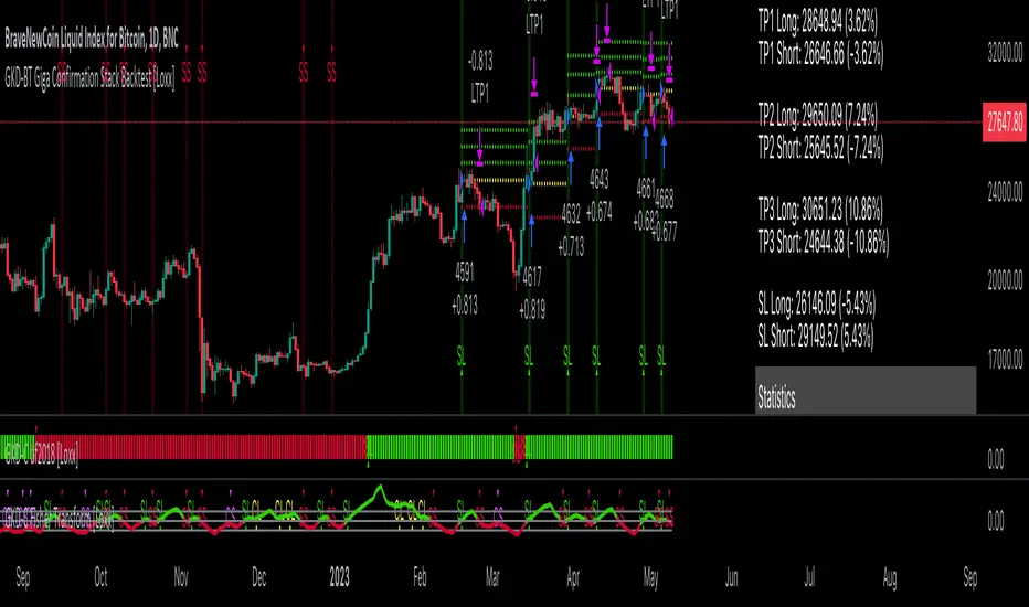
GKD-BT Giga Stacks Backtest [Loxx]Giga Kaleidoscope GKD-BT Giga Stacks Backtest is a Backtesting module included in Loxx's "Giga Kaleidoscope Modularized Trading System".
█ GKD-BT Giga Stacks Backtest
The Giga Stacks Backtest module allows users to perform backtesting on Long and Short signals from the confluence of GKD-B Baseline, GKD-C Confirmation, and GKD-V Volatility/Volume indicators. This module encompasses two types of backtests: Trading and Full. The Trading backtest permits users to evaluate individual trades, whether Long or Short, one at a time. Conversely, the Full backtest allows users to analyze either Longs or Shorts separately by toggling between them in the settings, enabling the examination of results for each signal type. The Trading backtest emulates actual trading conditions, while the Full backtest assesses all signals, regardless of being Long or Short.
Additionally, this backtest module provides the option to test using indicators with 1 to 3 take profits and 1 stop loss. The Trading backtest allows for the use of 1 to 3 take profits, while the Full backtest is limited to 1 take profit. The Trading backtest also offers the capability to apply a trailing take profit.
In terms of the percentage of trade removed at each take profit, this backtest module has the following hardcoded values:
Take profit 1: 50% of the trade is removed.
Take profit 2: 25% of the trade is removed.
Take profit 3: 25% of the trade is removed.
Stop loss: 100% of the trade is removed.
After each take profit is achieved, the stop loss level is adjusted. When take profit 1 is reached, the stop loss is moved to the entry point. Similarly, when take profit 2 is reached, the stop loss is shifted to take profit 1. The trailing take profit feature comes into play after take profit 2 or take profit 3, depending on the number of take profits selected in the settings. The trailing take profit is always activated on the final take profit when 2 or more take profits are chosen.
The backtest module also offers the capability to restrict by a specific date range, allowing for simulated forward testing based on past data. Additionally, users have the option to display or hide a trading panel that provides relevant information about the backtest, statistics, and the current trade. It is also possible to activate alerts and toggle sections of the trading panel on or off. On the chart, historical take profit and stop loss levels are represented by horizontal lines overlaid for reference.
To utilize this strategy, follow these steps (where "Stack XX" denotes the number of the Stack):
GKD-B Baseline Import: Import the value "Input into NEW GKD-BT Backtest" from the GKD-B Baseline module into the GKD-BT Giga Stacks Backtest module setting named "Stack XX: Import GKD-C, GKD-B, or GKD-V."
GKD-V Volatility/Volume Import: Import the value "Input into NEW GKD-BT Backtest" from the GKD-V Volatility/Volume module into the GKD-BT Giga Stacks Backtest module setting named "Stack XX: Import GKD-C, GKD-B, or GKD-V."
GKD-C Confirmation Import: 1) Adjust the "Confirmation Type" in the GKD-C Confirmation Indicator to "GKD New."; 2) Import the value "Input into NEW GKD-BT Backtest" from the GKD-C Confirmation module into the GKD-BT Giga Stacks Backtest module setting named "Stack XX: Import GKD-C, GKD-B, or GKD."
█ Giga Stacks Backtest Entries
Entries are generated form the confluence of up to six GKD-B Baseline, GKD-C Confirmation, and GKD-V Volatility/Volume indicators. Signals are generated when all Stacks reach uptrend or downtrend together.
Here's how this works. Assume we have the following Stacks and their respective trend on the current candle:
Stack 1 indicator is in uptreend
Stack 2 indicator is in downtrend
Stack 3 indicator is in uptreend
Stack 4 indicator is in uptreend
All stacks are in uptrend except for Stack 2. If Stack 2 reaches uptrend while Stacks 1, 3, and 4 stay in uptrend, then a long signal is generated. The last Stack to align with all other Stacks will generate a long or short signal.
█ Volatility Types Included
The GKD system utilizes volatility-based take profits and stop losses. Each take profit and stop loss is calculated as a multiple of volatility. Users can also adjust the multiplier values in the settings.
This module includes 17 types of volatility:
Close-to-Close
Parkinson
Garman-Klass
Rogers-Satchell
Yang-Zhang
Garman-Klass-Yang-Zhang
Exponential Weighted Moving Average
Standard Deviation of Log Returns
Pseudo GARCH(2,2)
Average True Range
True Range Double
Standard Deviation
Adaptive Deviation
Median Absolute Deviation
Efficiency-Ratio Adaptive ATR
Mean Absolute Deviation
Static Percent
Close-to-Close
Close-to-Close volatility is a classic and widely used volatility measure, sometimes referred to as historical volatility.
Volatility is an indicator of the speed of a stock price change. A stock with high volatility is one where the price changes rapidly and with a larger amplitude. The more volatile a stock is, the riskier it is.
Close-to-close historical volatility is calculated using only a stock's closing prices. It is the simplest volatility estimator. However, in many cases, it is not precise enough. Stock prices could jump significantly during a trading session and return to the opening value at the end. That means that a considerable amount of price information is not taken into account by close-to-close volatility.
Despite its drawbacks, Close-to-Close volatility is still useful in cases where the instrument doesn't have intraday prices. For example, mutual funds calculate their net asset values daily or weekly, and thus their prices are not suitable for more sophisticated volatility estimators.
Parkinson
Parkinson volatility is a volatility measure that uses the stock’s high and low price of the day.
The main difference between regular volatility and Parkinson volatility is that the latter uses high and low prices for a day, rather than only the closing price. This is useful as close-to-close prices could show little difference while large price movements could have occurred during the day. Thus, Parkinson's volatility is considered more precise and requires less data for calculation than close-to-close volatility.
One drawback of this estimator is that it doesn't take into account price movements after the market closes. Hence, it systematically undervalues volatility. This drawback is addressed in the Garman-Klass volatility estimator.
Garman-Klass
Garman-Klass is a volatility estimator that incorporates open, low, high, and close prices of a security.
Garman-Klass volatility extends Parkinson's volatility by taking into account the opening and closing prices. As markets are most active during the opening and closing of a trading session, it makes volatility estimation more accurate.
Garman and Klass also assumed that the process of price change follows a continuous diffusion process (Geometric Brownian motion). However, this assumption has several drawbacks. The method is not robust for opening jumps in price and trend movements.
Despite its drawbacks, the Garman-Klass estimator is still more effective than the basic formula since it takes into account not only the price at the beginning and end of the time interval but also intraday price extremes.
Researchers Rogers and Satchell have proposed a more efficient method for assessing historical volatility that takes into account price trends. See Rogers-Satchell Volatility for more detail.
Rogers-Satchell
Rogers-Satchell is an estimator for measuring the volatility of securities with an average return not equal to zero.
Unlike Parkinson and Garman-Klass estimators, Rogers-Satchell incorporates a drift term (mean return not equal to zero). As a result, it provides better volatility estimation when the underlying is trending.
The main disadvantage of this method is that it does not take into account price movements between trading sessions. This leads to an underestimation of volatility since price jumps periodically occur in the market precisely at the moments between sessions.
A more comprehensive estimator that also considers the gaps between sessions was developed based on the Rogers-Satchel formula in the 2000s by Yang-Zhang. See Yang Zhang Volatility for more detail.
Yang-Zhang
Yang Zhang is a historical volatility estimator that handles both opening jumps and the drift and has a minimum estimation error.
Yang-Zhang volatility can be thought of as a combination of the overnight (close-to-open volatility) and a weighted average of the Rogers-Satchell volatility and the day’s open-to-close volatility. It is considered to be 14 times more efficient than the close-to-close estimator.
Garman-Klass-Yang-Zhang
Garman-Klass-Yang-Zhang (GKYZ) volatility estimator incorporates the returns of open, high, low, and closing prices in its calculation.
GKYZ volatility estimator takes into account overnight jumps but not the trend, i.e., it assumes that the underlying asset follows a Geometric Brownian Motion (GBM) process with zero drift. Therefore, the GKYZ volatility estimator tends to overestimate the volatility when the drift is different from zero. However, for a GBM process, this estimator is eight times more efficient than the close-to-close volatility estimator.
Exponential Weighted Moving Average
The Exponentially Weighted Moving Average (EWMA) is a quantitative or statistical measure used to model or describe a time series. The EWMA is widely used in finance, with the main applications being technical analysis and volatility modeling.
The moving average is designed such that older observations are given lower weights. The weights decrease exponentially as the data point gets older – hence the name exponentially weighted.
The only decision a user of the EWMA must make is the parameter lambda. The parameter decides how important the current observation is in the calculation of the EWMA. The higher the value of lambda, the more closely the EWMA tracks the original time series.
Standard Deviation of Log Returns
This is the simplest calculation of volatility. It's the standard deviation of ln(close/close(1)).
Pseudo GARCH(2,2)
This is calculated using a short- and long-run mean of variance multiplied by ?.
?avg(var;M) + (1 ? ?) avg(var;N) = 2?var/(M+1-(M-1)L) + 2(1-?)var/(M+1-(M-1)L)
Solving for ? can be done by minimizing the mean squared error of estimation; that is, regressing L^-1var - avg(var; N) against avg(var; M) - avg(var; N) and using the resulting beta estimate as ?.
Average True Range
The average true range (ATR) is a technical analysis indicator, introduced by market technician J. Welles Wilder Jr. in his book New Concepts in Technical Trading Systems, that measures market volatility by decomposing the entire range of an asset price for that period.
The true range indicator is taken as the greatest of the following: current high less the current low; the absolute value of the current high less the previous close; and the absolute value of the current low less the previous close. The ATR is then a moving average, generally using 14 days, of the true ranges.
True Range Double
A special case of ATR that attempts to correct for volatility skew.
Standard Deviation
Standard deviation is a statistic that measures the dispersion of a dataset relative to its mean and is calculated as the square root of the variance. The standard deviation is calculated as the square root of variance by determining each data point's deviation relative to the mean. If the data points are further from the mean, there is a higher deviation within the data set; thus, the more spread out the data, the higher the standard deviation.
Adaptive Deviation
By definition, the Standard Deviation (STD, also represented by the Greek letter sigma ? or the Latin letter s) is a measure that is used to quantify the amount of variation or dispersion of a set of data values. In technical analysis, we usually use it to measure the level of current volatility.
Standard Deviation is based on Simple Moving Average calculation for mean value. This version of standard deviation uses the properties of EMA to calculate what can be called a new type of deviation, and since it is based on EMA, we can call it EMA deviation. Additionally, Perry Kaufman's efficiency ratio is used to make it adaptive (since all EMA type calculations are nearly perfect for adapting).
The difference when compared to the standard is significant--not just because of EMA usage, but the efficiency ratio makes it a "bit more logical" in very volatile market conditions.
Median Absolute Deviation
The median absolute deviation is a measure of statistical dispersion. Moreover, the MAD is a robust statistic, being more resilient to outliers in a data set than the standard deviation. In the standard deviation, the distances from the mean are squared, so large deviations are weighted more heavily, and thus outliers can heavily influence it. In the MAD, the deviations of a small number of outliers are irrelevant.
Because the MAD is a more robust estimator of scale than the sample variance or standard deviation, it works better with distributions without a mean or variance, such as the Cauchy distribution.
Efficiency-Ratio Adaptive ATR
Average True Range (ATR) is a widely used indicator for many occasions in technical analysis. It is calculated as the RMA of the true range. This version adds a "twist": it uses Perry Kaufman's Efficiency Ratio to calculate adaptive true range.
Mean Absolute Deviation
The mean absolute deviation (MAD) is a measure of variability that indicates the average distance between observations and their mean. MAD uses the original units of the data, which simplifies interpretation. Larger values signify that the data points spread out further from the average. Conversely, lower values correspond to data points bunching closer to it. The mean absolute deviation is also known as the mean deviation and average absolute deviation.
This definition of the mean absolute deviation sounds similar to the standard deviation (SD). While both measure variability, they have different calculations. In recent years, some proponents of MAD have suggested that it replace the SD as the primary measure because it is a simpler concept that better fits real life.
Static Percent
Static Percent allows the user to insert their own constant percent that will then be used to create take profits and stoploss
█ Giga Kaleidoscope Modularized Trading System
Core components of an NNFX algorithmic trading strategy
The NNFX algorithm is built on the principles of trend, momentum, and volatility. There are six core components in the NNFX trading algorithm:
1. Volatility - price volatility; e.g., Average True Range, True Range Double, Close-to-Close, etc.
2. Baseline - a moving average to identify price trend
3. Confirmation 1 - a technical indicator used to identify trends
4. Confirmation 2 - a technical indicator used to identify trends
5. Continuation - a technical indicator used to identify trends
6. Volatility/Volume - a technical indicator used to identify volatility/volume breakouts/breakdown
7. Exit - a technical indicator used to determine when a trend is exhausted
What is Volatility in the NNFX trading system?
In the NNFX (No Nonsense Forex) trading system, ATR (Average True Range) is typically used to measure the volatility of an asset. It is used as a part of the system to help determine the appropriate stop loss and take profit levels for a trade. ATR is calculated by taking the average of the true range values over a specified period.
True range is calculated as the maximum of the following values:
-Current high minus the current low
-Absolute value of the current high minus the previous close
-Absolute value of the current low minus the previous close
ATR is a dynamic indicator that changes with changes in volatility. As volatility increases, the value of ATR increases, and as volatility decreases, the value of ATR decreases. By using ATR in NNFX system, traders can adjust their stop loss and take profit levels according to the volatility of the asset being traded. This helps to ensure that the trade is given enough room to move, while also minimizing potential losses.
Other types of volatility include True Range Double (TRD), Close-to-Close, and Garman-Klass
What is a Baseline indicator?
The baseline is essentially a moving average, and is used to determine the overall direction of the market.
The baseline in the NNFX system is used to filter out trades that are not in line with the long-term trend of the market. The baseline is plotted on the chart along with other indicators, such as the Moving Average (MA), the Relative Strength Index (RSI), and the Average True Range (ATR).
Trades are only taken when the price is in the same direction as the baseline. For example, if the baseline is sloping upwards, only long trades are taken, and if the baseline is sloping downwards, only short trades are taken. This approach helps to ensure that trades are in line with the overall trend of the market, and reduces the risk of entering trades that are likely to fail.
By using a baseline in the NNFX system, traders can have a clear reference point for determining the overall trend of the market, and can make more informed trading decisions. The baseline helps to filter out noise and false signals, and ensures that trades are taken in the direction of the long-term trend.
What is a Confirmation indicator?
Confirmation indicators are technical indicators that are used to confirm the signals generated by primary indicators. Primary indicators are the core indicators used in the NNFX system, such as the Average True Range (ATR), the Moving Average (MA), and the Relative Strength Index (RSI).
The purpose of the confirmation indicators is to reduce false signals and improve the accuracy of the trading system. They are designed to confirm the signals generated by the primary indicators by providing additional information about the strength and direction of the trend.
Some examples of confirmation indicators that may be used in the NNFX system include the Bollinger Bands, the MACD (Moving Average Convergence Divergence), and the MACD Oscillator. These indicators can provide information about the volatility, momentum, and trend strength of the market, and can be used to confirm the signals generated by the primary indicators.
In the NNFX system, confirmation indicators are used in combination with primary indicators and other filters to create a trading system that is robust and reliable. By using multiple indicators to confirm trading signals, the system aims to reduce the risk of false signals and improve the overall profitability of the trades.
What is a Continuation indicator?
In the NNFX (No Nonsense Forex) trading system, a continuation indicator is a technical indicator that is used to confirm a current trend and predict that the trend is likely to continue in the same direction. A continuation indicator is typically used in conjunction with other indicators in the system, such as a baseline indicator, to provide a comprehensive trading strategy.
What is a Volatility/Volume indicator?
Volume indicators, such as the On Balance Volume (OBV), the Chaikin Money Flow (CMF), or the Volume Price Trend (VPT), are used to measure the amount of buying and selling activity in a market. They are based on the trading volume of the market, and can provide information about the strength of the trend. In the NNFX system, volume indicators are used to confirm trading signals generated by the Moving Average and the Relative Strength Index. Volatility indicators include Average Direction Index, Waddah Attar, and Volatility Ratio. In the NNFX trading system, volatility is a proxy for volume and vice versa.
By using volume indicators as confirmation tools, the NNFX trading system aims to reduce the risk of false signals and improve the overall profitability of trades. These indicators can provide additional information about the market that is not captured by the primary indicators, and can help traders to make more informed trading decisions. In addition, volume indicators can be used to identify potential changes in market trends and to confirm the strength of price movements.
What is an Exit indicator?
The exit indicator is used in conjunction with other indicators in the system, such as the Moving Average (MA), the Relative Strength Index (RSI), and the Average True Range (ATR), to provide a comprehensive trading strategy.
The exit indicator in the NNFX system can be any technical indicator that is deemed effective at identifying optimal exit points. Examples of exit indicators that are commonly used include the Parabolic SAR, the Average Directional Index (ADX), and the Chandelier Exit.
The purpose of the exit indicator is to identify when a trend is likely to reverse or when the market conditions have changed, signaling the need to exit a trade. By using an exit indicator, traders can manage their risk and prevent significant losses.
In the NNFX system, the exit indicator is used in conjunction with a stop loss and a take profit order to maximize profits and minimize losses. The stop loss order is used to limit the amount of loss that can be incurred if the trade goes against the trader, while the take profit order is used to lock in profits when the trade is moving in the trader's favor.
Overall, the use of an exit indicator in the NNFX trading system is an important component of a comprehensive trading strategy. It allows traders to manage their risk effectively and improve the profitability of their trades by exiting at the right time.
How does Loxx's GKD (Giga Kaleidoscope Modularized Trading System) implement the NNFX algorithm outlined above?
Loxx's GKD v2.0 system has five types of modules (indicators/strategies). These modules are:
1. GKD-BT - Backtesting module (Volatility, Number 1 in the NNFX algorithm)
2. GKD-B - Baseline module (Baseline and Volatility/Volume, Numbers 1 and 2 in the NNFX algorithm)
3. GKD-C - Confirmation 1/2 and Continuation module (Confirmation 1/2 and Continuation, Numbers 3, 4, and 5 in the NNFX algorithm)
4. GKD-V - Volatility/Volume module (Confirmation 1/2, Number 6 in the NNFX algorithm)
5. GKD-E - Exit module (Exit, Number 7 in the NNFX algorithm)
(additional module types will added in future releases)
Each module interacts with every module by passing data to A backtest module wherein the various components of the GKD system are combined to create a trading signal.
That is, the Baseline indicator passes its data to Volatility/Volume. The Volatility/Volume indicator passes its values to the Confirmation 1 indicator. The Confirmation 1 indicator passes its values to the Confirmation 2 indicator. The Confirmation 2 indicator passes its values to the Continuation indicator. The Continuation indicator passes its values to the Exit indicator, and finally, the Exit indicator passes its values to the Backtest strategy.
This chaining of indicators requires that each module conform to Loxx's GKD protocol, therefore allowing for the testing of every possible combination of technical indicators that make up the six components of the NNFX algorithm.
What does the application of the GKD trading system look like?
Example trading system:
Backtest: Stacks Backtest
Baseline: Hull Moving Average
Volatility/Volume: Hurst Exponent
Confirmation 1: Vorext
Confirmation 2: Coppock Curve
Continuation: Fisher Transform
Exit: Rex Oscillator
Each GKD indicator is denoted with a module identifier of either: GKD-BT, GKD-B, GKD-C, GKD-V, or GKD-E. This allows traders to understand to which module each indicator belongs and where each indicator fits into the GKD system.

GKD-BT Full Giga Kaleidoscope Backtest [Loxx]Giga Kaleidoscope GKD-BT Full Giga Kaleidoscope Backtest is a Backtesting module included in Loxx's "Giga Kaleidoscope Modularized Trading System".
█ GKD-BT Full Giga Kaleidoscope Backtest
The Full Giga Kaleidoscope Backtest module enables users to backtest Full GKD Long and Short signals, allowing the creation of a comprehensive NNFX trading system consisting of two confirmation indicators, a baseline, a measure of volatility/volume, and continuations.
This module offers two types of backtests: Trading and Full. The Trading backtest allows users to evaluate individual Long and Short trades one by one. On the other hand, the Full backtest enables the analysis of Longs or Shorts separately by toggling between them in the settings, providing insights into the results for each signal type. The Trading backtest simulates actual trading conditions, while the Full backtest evaluates all signals regardless of their Long or Short nature.
Additionally, the backtest module allows testing with 1 to 3 take profits and 1 stop loss. The Trading backtest supports 1 to 3 take profits, while the Full backtest is limited to 1 take profit. The Trading backtest also includes a trailing take profit feature.
Regarding the percentage of trade removed at each take profit, the backtest module incorporates the following predefined values:
Take profit 1: 50% of the trade is removed.
Take profit 2: 25% of the trade is removed.
Take profit 3: 25% of the trade is removed.
Stop loss: 100% of the trade is removed.
After achieving each take profit, the stop loss level is adjusted accordingly. When take profit 1 is reached, the stop loss is moved to the entry point. Similarly, when take profit 2 is reached, the stop loss is shifted to take profit 1. The trailing take profit feature comes into effect after take profit 2 or take profit 3, depending on the number of take profits selected in the settings. The trailing take profit is always activated on the final take profit when 2 or more take profits are chosen.
The backtest module also provides the option to restrict testing to a specific date range, allowing for simulated forward testing using past data. Additionally, users can choose to display or hide a trading panel that provides relevant information about the backtest, statistics, and the current trade. It is also possible to activate alerts and toggle sections of the trading panel on or off. Historical take profit and stop loss levels are displayed as overlaid horizontal lines on the chart for reference.
To utilize this strategy, follow these steps:
1. GKD-B Baseline Import: Import the value "Input into NEW GKD-BT Backtest" from the GKD-B Baseline module into the GKD-BT Full Giga Kaleidoscope Backtest module setting named "Import GKD-B Baseline."
2. GKD-V Volatility/Volume Import: Import the value "Input into NEW GKD-BT Backtest" from the GKD-V Volatility/Volume module into the GKD-BT Full Giga Kaleidoscope Backtest module setting named "Import GKD-V Volatility/Volume."
3. Adjust the "Confirmation 1 Type" in the GKD-C Confirmation Indicator to "GKD New."
4. GKD-C Confirmation 1 Import: Import the value "Input into NEW GKD-BT Backtest" from the GKD-C Confirmation 1 module into the GKD-BT Full Giga Kaleidoscope Backtest module setting named "Import GKD-C Confirmation 1."
5. Adjust the "Confirmation 2 Type" in the GKD-C Confirmation 2 Indicator to "GKD New."
6. GKD-C Confirmation 2 Import: Import the value "Input into NEW GKD-BT Backtest" from the GKD-C Confirmation 2 module into the GKD-BT Full Giga Kaleidoscope Backtest module setting named "Import GKD-C Confirmation 2."
7. Adjust the "Confirmation Type" in the GKD-C Continuation Indicator to "GKD New."
8. GKD-C Continuation Import: Import the value "Input into NEW GKD-BT Backtest" from the GKD-C Continuation module into the GKD-BT Full Giga Kaleidoscope Backtest module setting named "Import GKD-C Confirmation."
The GKD system utilizes volatility-based take profits and stop losses, where each take profit and stop loss is calculated as a multiple of volatility. Users have the flexibility to adjust the multiplier values in the settings to suit their preferences.
In a future update, the Full Giga Kaleidoscope Backtest module will include the option to incorporate a GKD-E Exit indicator, completing the full trading strategy.
█ Full Giga Kaleidoscope Backtest Entries
Within this module, there are ten distinct types of entries available, which are outlined below:
Standard Entry
1-Candle Standard Entry
Baseline Entry
1-Candle Baseline Entry
Volatility/Volume Entry
1-Candle Volatility/Volume Entry
Confirmation 2 Entry
1-Candle Confirmation 2 Entry
PullBack Entry
Continuation Entry
Each of these entry types can generate either long or short signals, resulting in a total of 20 signal variations. The user has the flexibility to enable or disable specific entry types and choose which qualifying rules within each entry type are applied to price to determine the final long or short signal.
The following section provides an overview of the various entry types and their corresponding qualifying rules:
Standard Entry
1. GKD-C Confirmation gives signal
2. Baseline agrees
3. Price inside Goldie Locks Zone Minimum
4. Price inside Goldie Locks Zone Maximum
5. Confirmation 2 agrees
6. Volatility/Volume agrees
1-Candle Standard Entry
1a. GKD-C Confirmation gives signal
2a. Baseline agrees
3a. Price inside Goldie Locks Zone Minimum
4a. Price inside Goldie Locks Zone Maximum
Next Candle
1b. Price retraced
2b. Baseline agrees
3b. Confirmation 1 agrees
4b. Confirmation 2 agrees
5b. Volatility/Volume agrees
Baseline Entry
1. GKD-B Basline gives signal
2. Confirmation 1 agrees
3. Price inside Goldie Locks Zone Minimum
4. Price inside Goldie Locks Zone Maximum
5. Confirmation 2 agrees
6. Volatility/Volume agrees
7. Confirmation 1 signal was less than 'Maximum Allowable PSBC Bars Back' prior
1-Candle Baseline Entry
1a. GKD-B Baseline gives signal
2a. Confirmation 1 agrees
3a. Price inside Goldie Locks Zone Minimum
4a. Price inside Goldie Locks Zone Maximum
5a. Confirmation 1 signal was less than 'Maximum Allowable PSBC Bars Back' prior
Next Candle
1b. Price retraced
2b. Baseline agrees
3b. Confirmation 1 agrees
4b. Confirmation 2 agrees
5b. Volatility/Volume agrees
Volatility/Volume Entry
1. GKD-V Volatility/Volume gives signal
2. Confirmation 1 agrees
3. Price inside Goldie Locks Zone Minimum
4. Price inside Goldie Locks Zone Maximum
5. Confirmation 2 agrees
6. Baseline agrees
7. Confirmation 1 signal was less than 7 candles prior
1-Candle Volatility/Volume Entry
1a. GKD-V Volatility/Volume gives signal
2a. Confirmation 1 agrees
3a. Price inside Goldie Locks Zone Minimum
4a. Price inside Goldie Locks Zone Maximum
5a. Confirmation 1 signal was less than 'Maximum Allowable PSVVC Bars Back' prior
Next Candle
1b. Price retraced
2b. Volatility/Volume agrees
3b. Confirmation 1 agrees
4b. Confirmation 2 agrees
5b. Baseline agrees
Confirmation 2 Entry
1. GKD-C Confirmation 2 gives signal
2. Confirmation 1 agrees
3. Price inside Goldie Locks Zone Minimum
4. Price inside Goldie Locks Zone Maximum
5. Volatility/Volume agrees
6. Baseline agrees
7. Confirmation 1 signal was less than 7 candles prior
1-Candle Confirmation 2 Entry
1a. GKD-C Confirmation 2 gives signal
2a. Confirmation 1 agrees
3a. Price inside Goldie Locks Zone Minimum
4a. Price inside Goldie Locks Zone Maximum
5a. Confirmation 1 signal was less than 'Maximum Allowable PSC2C Bars Back' prior
Next Candle
1b. Price retraced
2b. Confirmation 2 agrees
3b. Confirmation 1 agrees
4b. Volatility/Volume agrees
5b. Baseline agrees
PullBack Entry
1a. GKD-B Baseline gives signal
2a. Confirmation 1 agrees
3a. Price is beyond 1.0x Volatility of Baseline
Next Candle
1b. Price inside Goldie Locks Zone Minimum
2b. Price inside Goldie Locks Zone Maximum
3b. Confirmation 1 agrees
4b. Confirmation 2 agrees
5b. Volatility/Volume agrees
Continuation Entry
1. Standard Entry, 1-Candle Standard Entry, Baseline Entry, 1-Candle Baseline Entry, Volatility/Volume Entry, 1-Candle Volatility/Volume Entry, Confirmation 2 Entry, 1-Candle Confirmation 2 Entry, or Pullback entry triggered previously
2. Baseline hasn't crossed since entry signal trigger
4. Confirmation 1 agrees
5. Baseline agrees
6. Confirmation 2 agrees
█ Volatility Types Included
This module includes 17 types of volatility:
Close-to-Close
Parkinson
Garman-Klass
Rogers-Satchell
Yang-Zhang
Garman-Klass-Yang-Zhang
Exponential Weighted Moving Average
Standard Deviation of Log Returns
Pseudo GARCH(2,2)
Average True Range
True Range Double
Standard Deviation
Adaptive Deviation
Median Absolute Deviation
Efficiency-Ratio Adaptive ATR
Mean Absolute Deviation
Static Percent
Close-to-Close
Close-to-Close volatility is a classic and widely used volatility measure, sometimes referred to as historical volatility.
Volatility is an indicator of the speed of a stock price change. A stock with high volatility is one where the price changes rapidly and with a larger amplitude. The more volatile a stock is, the riskier it is.
Close-to-close historical volatility is calculated using only a stock's closing prices. It is the simplest volatility estimator. However, in many cases, it is not precise enough. Stock prices could jump significantly during a trading session and return to the opening value at the end. That means that a considerable amount of price information is not taken into account by close-to-close volatility.
Despite its drawbacks, Close-to-Close volatility is still useful in cases where the instrument doesn't have intraday prices. For example, mutual funds calculate their net asset values daily or weekly, and thus their prices are not suitable for more sophisticated volatility estimators.
Parkinson
Parkinson volatility is a volatility measure that uses the stock’s high and low price of the day.
The main difference between regular volatility and Parkinson volatility is that the latter uses high and low prices for a day, rather than only the closing price. This is useful as close-to-close prices could show little difference while large price movements could have occurred during the day. Thus, Parkinson's volatility is considered more precise and requires less data for calculation than close-to-close volatility.
One drawback of this estimator is that it doesn't take into account price movements after the market closes. Hence, it systematically undervalues volatility. This drawback is addressed in the Garman-Klass volatility estimator.
Garman-Klass
Garman-Klass is a volatility estimator that incorporates open, low, high, and close prices of a security.
Garman-Klass volatility extends Parkinson's volatility by taking into account the opening and closing prices. As markets are most active during the opening and closing of a trading session, it makes volatility estimation more accurate.
Garman and Klass also assumed that the process of price change follows a continuous diffusion process (Geometric Brownian motion). However, this assumption has several drawbacks. The method is not robust for opening jumps in price and trend movements.
Despite its drawbacks, the Garman-Klass estimator is still more effective than the basic formula since it takes into account not only the price at the beginning and end of the time interval but also intraday price extremes.
Researchers Rogers and Satchell have proposed a more efficient method for assessing historical volatility that takes into account price trends. See Rogers-Satchell Volatility for more detail.
Rogers-Satchell
Rogers-Satchell is an estimator for measuring the volatility of securities with an average return not equal to zero.
Unlike Parkinson and Garman-Klass estimators, Rogers-Satchell incorporates a drift term (mean return not equal to zero). As a result, it provides better volatility estimation when the underlying is trending.
The main disadvantage of this method is that it does not take into account price movements between trading sessions. This leads to an underestimation of volatility since price jumps periodically occur in the market precisely at the moments between sessions.
A more comprehensive estimator that also considers the gaps between sessions was developed based on the Rogers-Satchel formula in the 2000s by Yang-Zhang. See Yang Zhang Volatility for more detail.
Yang-Zhang
Yang Zhang is a historical volatility estimator that handles both opening jumps and the drift and has a minimum estimation error.
Yang-Zhang volatility can be thought of as a combination of the overnight (close-to-open volatility) and a weighted average of the Rogers-Satchell volatility and the day’s open-to-close volatility. It is considered to be 14 times more efficient than the close-to-close estimator.
Garman-Klass-Yang-Zhang
Garman-Klass-Yang-Zhang (GKYZ) volatility estimator incorporates the returns of open, high, low, and closing prices in its calculation.
GKYZ volatility estimator takes into account overnight jumps but not the trend, i.e., it assumes that the underlying asset follows a Geometric Brownian Motion (GBM) process with zero drift. Therefore, the GKYZ volatility estimator tends to overestimate the volatility when the drift is different from zero. However, for a GBM process, this estimator is eight times more efficient than the close-to-close volatility estimator.
Exponential Weighted Moving Average
The Exponentially Weighted Moving Average (EWMA) is a quantitative or statistical measure used to model or describe a time series. The EWMA is widely used in finance, with the main applications being technical analysis and volatility modeling.
The moving average is designed such that older observations are given lower weights. The weights decrease exponentially as the data point gets older – hence the name exponentially weighted.
The only decision a user of the EWMA must make is the parameter lambda. The parameter decides how important the current observation is in the calculation of the EWMA. The higher the value of lambda, the more closely the EWMA tracks the original time series.
Standard Deviation of Log Returns
This is the simplest calculation of volatility. It's the standard deviation of ln(close/close(1)).
Pseudo GARCH(2,2)
This is calculated using a short- and long-run mean of variance multiplied by ?.
?avg(var;M) + (1 ? ?) avg(var;N) = 2?var/(M+1-(M-1)L) + 2(1-?)var/(M+1-(M-1)L)
Solving for ? can be done by minimizing the mean squared error of estimation; that is, regressing L^-1var - avg(var; N) against avg(var; M) - avg(var; N) and using the resulting beta estimate as ?.
Average True Range
The average true range (ATR) is a technical analysis indicator, introduced by market technician J. Welles Wilder Jr. in his book New Concepts in Technical Trading Systems, that measures market volatility by decomposing the entire range of an asset price for that period.
The true range indicator is taken as the greatest of the following: current high less the current low; the absolute value of the current high less the previous close; and the absolute value of the current low less the previous close. The ATR is then a moving average, generally using 14 days, of the true ranges.
True Range Double
A special case of ATR that attempts to correct for volatility skew.
Standard Deviation
Standard deviation is a statistic that measures the dispersion of a dataset relative to its mean and is calculated as the square root of the variance. The standard deviation is calculated as the square root of variance by determining each data point's deviation relative to the mean. If the data points are further from the mean, there is a higher deviation within the data set; thus, the more spread out the data, the higher the standard deviation.
Adaptive Deviation
By definition, the Standard Deviation (STD, also represented by the Greek letter sigma ? or the Latin letter s) is a measure that is used to quantify the amount of variation or dispersion of a set of data values. In technical analysis, we usually use it to measure the level of current volatility.
Standard Deviation is based on Simple Moving Average calculation for mean value. This version of standard deviation uses the properties of EMA to calculate what can be called a new type of deviation, and since it is based on EMA, we can call it EMA deviation. Additionally, Perry Kaufman's efficiency ratio is used to make it adaptive (since all EMA type calculations are nearly perfect for adapting).
The difference when compared to the standard is significant--not just because of EMA usage, but the efficiency ratio makes it a "bit more logical" in very volatile market conditions.
Median Absolute Deviation
The median absolute deviation is a measure of statistical dispersion. Moreover, the MAD is a robust statistic, being more resilient to outliers in a data set than the standard deviation. In the standard deviation, the distances from the mean are squared, so large deviations are weighted more heavily, and thus outliers can heavily influence it. In the MAD, the deviations of a small number of outliers are irrelevant.
Because the MAD is a more robust estimator of scale than the sample variance or standard deviation, it works better with distributions without a mean or variance, such as the Cauchy distribution.
Efficiency-Ratio Adaptive ATR
Average True Range (ATR) is a widely used indicator for many occasions in technical analysis. It is calculated as the RMA of the true range. This version adds a "twist": it uses Perry Kaufman's Efficiency Ratio to calculate adaptive true range.
Mean Absolute Deviation
The mean absolute deviation (MAD) is a measure of variability that indicates the average distance between observations and their mean. MAD uses the original units of the data, which simplifies interpretation. Larger values signify that the data points spread out further from the average. Conversely, lower values correspond to data points bunching closer to it. The mean absolute deviation is also known as the mean deviation and average absolute deviation.
This definition of the mean absolute deviation sounds similar to the standard deviation (SD). While both measure variability, they have different calculations. In recent years, some proponents of MAD have suggested that it replace the SD as the primary measure because it is a simpler concept that better fits real life.
Static Percent
Static Percent allows the user to insert their own constant percent that will then be used to create take profits and stoploss
█ Giga Kaleidoscope Modularized Trading System
Core components of an NNFX algorithmic trading strategy
The NNFX algorithm is built on the principles of trend, momentum, and volatility. There are six core components in the NNFX trading algorithm:
1. Volatility - price volatility; e.g., Average True Range, True Range Double, Close-to-Close, etc.
2. Baseline - a moving average to identify price trend
3. Confirmation 1 - a technical indicator used to identify trends
4. Confirmation 2 - a technical indicator used to identify trends
5. Continuation - a technical indicator used to identify trends
6. Volatility/Volume - a technical indicator used to identify volatility/volume breakouts/breakdown
7. Exit - a technical indicator used to determine when a trend is exhausted
What is Volatility in the NNFX trading system?
In the NNFX (No Nonsense Forex) trading system, ATR (Average True Range) is typically used to measure the volatility of an asset. It is used as a part of the system to help determine the appropriate stop loss and take profit levels for a trade. ATR is calculated by taking the average of the true range values over a specified period.
True range is calculated as the maximum of the following values:
-Current high minus the current low
-Absolute value of the current high minus the previous close
-Absolute value of the current low minus the previous close
ATR is a dynamic indicator that changes with changes in volatility. As volatility increases, the value of ATR increases, and as volatility decreases, the value of ATR decreases. By using ATR in NNFX system, traders can adjust their stop loss and take profit levels according to the volatility of the asset being traded. This helps to ensure that the trade is given enough room to move, while also minimizing potential losses.
Other types of volatility include True Range Double (TRD), Close-to-Close, and Garman-Klass
What is a Baseline indicator?
The baseline is essentially a moving average, and is used to determine the overall direction of the market.
The baseline in the NNFX system is used to filter out trades that are not in line with the long-term trend of the market. The baseline is plotted on the chart along with other indicators, such as the Moving Average (MA), the Relative Strength Index (RSI), and the Average True Range (ATR).
Trades are only taken when the price is in the same direction as the baseline. For example, if the baseline is sloping upwards, only long trades are taken, and if the baseline is sloping downwards, only short trades are taken. This approach helps to ensure that trades are in line with the overall trend of the market, and reduces the risk of entering trades that are likely to fail.
By using a baseline in the NNFX system, traders can have a clear reference point for determining the overall trend of the market, and can make more informed trading decisions. The baseline helps to filter out noise and false signals, and ensures that trades are taken in the direction of the long-term trend.
What is a Confirmation indicator?
Confirmation indicators are technical indicators that are used to confirm the signals generated by primary indicators. Primary indicators are the core indicators used in the NNFX system, such as the Average True Range (ATR), the Moving Average (MA), and the Relative Strength Index (RSI).
The purpose of the confirmation indicators is to reduce false signals and improve the accuracy of the trading system. They are designed to confirm the signals generated by the primary indicators by providing additional information about the strength and direction of the trend.
Some examples of confirmation indicators that may be used in the NNFX system include the Bollinger Bands, the MACD (Moving Average Convergence Divergence), and the MACD Oscillator. These indicators can provide information about the volatility, momentum, and trend strength of the market, and can be used to confirm the signals generated by the primary indicators.
In the NNFX system, confirmation indicators are used in combination with primary indicators and other filters to create a trading system that is robust and reliable. By using multiple indicators to confirm trading signals, the system aims to reduce the risk of false signals and improve the overall profitability of the trades.
What is a Continuation indicator?
In the NNFX (No Nonsense Forex) trading system, a continuation indicator is a technical indicator that is used to confirm a current trend and predict that the trend is likely to continue in the same direction. A continuation indicator is typically used in conjunction with other indicators in the system, such as a baseline indicator, to provide a comprehensive trading strategy.
What is a Volatility/Volume indicator?
Volume indicators, such as the On Balance Volume (OBV), the Chaikin Money Flow (CMF), or the Volume Price Trend (VPT), are used to measure the amount of buying and selling activity in a market. They are based on the trading volume of the market, and can provide information about the strength of the trend. In the NNFX system, volume indicators are used to confirm trading signals generated by the Moving Average and the Relative Strength Index. Volatility indicators include Average Direction Index, Waddah Attar, and Volatility Ratio. In the NNFX trading system, volatility is a proxy for volume and vice versa.
By using volume indicators as confirmation tools, the NNFX trading system aims to reduce the risk of false signals and improve the overall profitability of trades. These indicators can provide additional information about the market that is not captured by the primary indicators, and can help traders to make more informed trading decisions. In addition, volume indicators can be used to identify potential changes in market trends and to confirm the strength of price movements.
What is an Exit indicator?
The exit indicator is used in conjunction with other indicators in the system, such as the Moving Average (MA), the Relative Strength Index (RSI), and the Average True Range (ATR), to provide a comprehensive trading strategy.
The exit indicator in the NNFX system can be any technical indicator that is deemed effective at identifying optimal exit points. Examples of exit indicators that are commonly used include the Parabolic SAR, the Average Directional Index (ADX), and the Chandelier Exit.
The purpose of the exit indicator is to identify when a trend is likely to reverse or when the market conditions have changed, signaling the need to exit a trade. By using an exit indicator, traders can manage their risk and prevent significant losses.
In the NNFX system, the exit indicator is used in conjunction with a stop loss and a take profit order to maximize profits and minimize losses. The stop loss order is used to limit the amount of loss that can be incurred if the trade goes against the trader, while the take profit order is used to lock in profits when the trade is moving in the trader's favor.
Overall, the use of an exit indicator in the NNFX trading system is an important component of a comprehensive trading strategy. It allows traders to manage their risk effectively and improve the profitability of their trades by exiting at the right time.
How does Loxx's GKD (Giga Kaleidoscope Modularized Trading System) implement the NNFX algorithm outlined above?
Loxx's GKD v2.0 system has five types of modules (indicators/strategies). These modules are:
1. GKD-BT - Backtesting module (Volatility, Number 1 in the NNFX algorithm)
2. GKD-B - Baseline module (Baseline and Volatility/Volume, Numbers 1 and 2 in the NNFX algorithm)
3. GKD-C - Confirmation 1/2 and Continuation module (Confirmation 1/2 and Continuation, Numbers 3, 4, and 5 in the NNFX algorithm)
4. GKD-V - Volatility/Volume module (Confirmation 1/2, Number 6 in the NNFX algorithm)
5. GKD-E - Exit module (Exit, Number 7 in the NNFX algorithm)
(additional module types will added in future releases)
Each module interacts with every module by passing data to A backtest module wherein the various components of the GKD system are combined to create a trading signal.
That is, the Baseline indicator passes its data to Volatility/Volume. The Volatility/Volume indicator passes its values to the Confirmation 1 indicator. The Confirmation 1 indicator passes its values to the Confirmation 2 indicator. The Confirmation 2 indicator passes its values to the Continuation indicator. The Continuation indicator passes its values to the Exit indicator, and finally, the Exit indicator passes its values to the Backtest strategy.
This chaining of indicators requires that each module conform to Loxx's GKD protocol, therefore allowing for the testing of every possible combination of technical indicators that make up the six components of the NNFX algorithm.
What does the application of the GKD trading system look like?
Example trading system:
Backtest: Full Giga Kaleidoscope Backtest as shown on the chart above
Baseline: Hull Moving Average as shown on the chart above
Volatility/Volume: Hurst Exponent as shown on the chart above
Confirmation 1: Vorext as shown on the chart above
Confirmation 2: Coppock Curve as shown on the chart above
Continuation: Fisher Transform as shown on the chart above
Exit: Rex Oscillator
Each GKD indicator is denoted with a module identifier of either: GKD-BT, GKD-B, GKD-C, GKD-V, or GKD-E. This allows traders to understand to which module each indicator belongs and where each indicator fits into the GKD system.
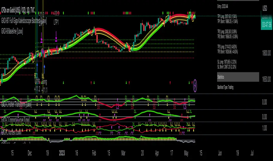
GKD-BT Solo Confirmation Super Complex Backtest [Loxx]Giga Kaleidoscope GKD-BT Solo Confirmation Super Complex Backtest is a Backtesting module included in Loxx's "Giga Kaleidoscope Modularized Trading System".
█ GKD-BT Solo Confirmation Super Complex Backtest
The Solo Confirmation Super Complex Backtest module allows users to perform backtesting on Full GKD Long and Short signals using GKD-C confirmation indicators. These signals are further refined by GKD-B Baseline and GKD-V Volatility/Volume indicators and augmented by an additional GKD-C Confirmation indicator acting as a Continuation indicator. This module serves as a comprehensive tool that falls just below a Full GKD trading system. The key difference is that the GKD-BT Solo Confirmation Super Complex utilizes a single GKD-C Confirmation indicator, while the Full GKD system employs two GKD-C Confirmation indicators. Both the Solo Confirmation Super Complex and the Full GKD systems incorporate an extra GKD-C Confirmation indicator to identify Continuation signals, which provide both longs and shorts on developing trends following an initial trend change.
This module encompasses two types of backtests: Trading and Full. The Trading backtest permits users to evaluate individual trades, whether Long or Short, one at a time. Conversely, the Full backtest allows users to analyze either Longs or Shorts separately by toggling between them in the settings, enabling the examination of results for each signal type. The Trading backtest emulates actual trading conditions, while the Full backtest assesses all signals, regardless of being Long or Short.
Additionally, this backtest module provides the option to test the core GKD-C Confirmation and GKD-C Continuation indicators with 1 to 3 take profits and 1 stop loss. The Trading backtest allows for the use of 1 to 3 take profits, while the Full backtest is limited to 1 take profit. The Trading backtest also offers the capability to apply a trailing take profit.
In terms of the percentage of trade removed at each take profit, this backtest module has the following hardcoded values:
Take profit 1: 50% of the trade is removed.
Take profit 2: 25% of the trade is removed.
Take profit 3: 25% of the trade is removed.
Stop loss: 100% of the trade is removed.
After each take profit is achieved, the stop loss level is adjusted. When take profit 1 is reached, the stop loss is moved to the entry point. Similarly, when take profit 2 is reached, the stop loss is shifted to take profit 1. The trailing take profit feature comes into play after take profit 2 or take profit 3, depending on the number of take profits selected in the settings. The trailing take profit is always activated on the final take profit when 2 or more take profits are chosen.
The backtest module also offers the capability to restrict by a specific date range, allowing for simulated forward testing based on past data. Additionally, users have the option to display or hide a trading panel that provides relevant information about the backtest, statistics, and the current trade. It is also possible to activate alerts and toggle sections of the trading panel on or off. On the chart, historical take profit and stop loss levels are represented by horizontal lines overlaid for reference.
To utilize this strategy, follow these steps:
1. GKD-B Baseline Import: Import the value "Input into NEW GKD-BT Backtest" from the GKD-B Baseline module into the GKD-BT Solo Confirmation Super Complex Backtest module setting named "Import GKD-B Baseline."
2. GKD-V Volatility/Volume Import: Import the value "Input into NEW GKD-BT Backtest" from the GKD-V Volatility/Volume module into the GKD-BT Solo Confirmation Super Complex Backtest module setting named "Import GKD-V Volatility/Volume."
3. Adjust the "Confirmation Type" in the GKD-C Confirmation Indicator to "GKD New."
4. GKD-C Confirmation Import: Import the value "Input into NEW GKD-BT Backtest" from the GKD-C Confirmation module into the GKD-BT Solo Confirmation Super Complex Backtest module setting named "Import GKD-C Confirmation."
5. Adjust the "Confirmation Type" in the GKD-C Continuation Indicator to "GKD New."
6. GKD-C Continuation Import: Import the value "Input into NEW GKD-BT Backtest" from the GKD-C Continuation module into the GKD-BT Solo Confirmation Super Complex Backtest module setting named "Import GKD-C Continuation."
The GKD system utilizes volatility-based take profits and stop losses. Each take profit and stop loss is calculated as a multiple of volatility. Users can also adjust the multiplier values in the settings.
In a future update, the option to include a GKD-E Exit indicator will be added to this module to complete a full trading strategy.
█ Solo Confirmation Super Complex Backtest Entries
Within this module, there are eight distinct types of entries available, which are outlined below:
Standard Entry
1-Candle Standard Entry
Baseline Entry
1-Candle Baseline Entry
Volatility/Volume Entry
1-Candle Volatility/Volume Entry
PullBack Entry
Continuation Entry
Each of these entry types can generate either long or short signals, resulting in a total of 16 signal variations. The user has the flexibility to enable or disable specific entry types and choose which qualifying rules within each entry type are applied to price to determine the final long or short signal. You'll notice that these signals are different form the core GKD signals mentioned towards the end of this description. Signals from the GKD-BT Solo Confirmation Super Complex Backtest are modifided to add additional qualifications to make your finalized trading strategy more dynamic and robust.
The following section provides an overview of the various entry types and their corresponding qualifying rules:
Standard Entry
1. GKD-C Confirmation gives signal
2. Baseline agrees
3. Price inside Goldie Locks Zone Minimum
4. Price inside Goldie Locks Zone Maximum
5. Volatility/Volume agrees
1-Candle Standard Entry
1a. GKD-C Confirmation gives signal
2a. Baseline agrees
3a. Price inside Goldie Locks Zone Minimum
4a. Price inside Goldie Locks Zone Maximum
Next Candle:
1b. Price retraced
2b. Baseline agrees
3b. Confirmation 1 agrees
4b. Volatility/Volume agrees
Baseline Entry
1. GKD-B Basline gives signal
2. Confirmation 1 agrees
3. Price inside Goldie Locks Zone Minimum
4. Price inside Goldie Locks Zone Maximum
5. Volatility/Volume agrees
6. Confirmation 1 signal was less than 'Maximum Allowable PSBC Bars Back' prior
1-Candle Baseline Entry
1a. GKD-B Basline gives signal
2a. Confirmation 1 agrees
3a. Price inside Goldie Locks Zone Minimum
4a. Price inside Goldie Locks Zone Maximum
5a. Confirmation 1 signal was less than 'Maximum Allowable PSBC Bars Back' prior
Next Candle:
1b. Price retraced
2b. Baseline agrees
3b. Confirmation 1 agrees
4b. Volatility/Volume agrees
Volatility/Volume Entry
1. GKD-V Volatility/Volume gives signal
2. Confirmation 1 agrees
3. Price inside Goldie Locks Zone Minimum
4. Price inside Goldie Locks Zone Maximum
5. Baseline agrees
6. Confirmation 1 signal was less than 7 candles prior
1-Candle Volatility/Volume Entry
1a. GKD-V Volatility/Volume gives signal
2a. Confirmation 1 agrees
3a. Price inside Goldie Locks Zone Minimum
4a. Price inside Goldie Locks Zone Maximum
5a. Confirmation 1 signal was less than 'Maximum Allowable PSVVC Bars Back' prior
Next Candle:
1b. Price retraced
2b. Volatility/Volume agrees
3b. Confirmation 1 agrees
4b. Baseline agrees
PullBack Entry
1a. GKD-B Baseline gives signal
2a. Confirmation 1 agrees
3a. Price is beyond 1.0x Volatility of Baseline
Next Candle:
1b. Price inside Goldie Locks Zone Minimum
2b. Price inside Goldie Locks Zone Maximum
3b. Confirmation 1 agrees
4b. Volatility/Volume agrees
Continuation Entry
1. Standard Entry, 1-Candle Standard Entry, Baseline Entry, 1-Candle Baseline Entry, Volatility/Volume Entry, 1-Candle Volatility/Volume Entry, or Pullback entry triggered previously
2. Baseline hasn't crossed since entry signal trigger
4. Confirmation 1 agrees
5. Baseline agrees
█ Volatility Types Included
This module includes 17 types of volatility:
Close-to-Close
Parkinson
Garman-Klass
Rogers-Satchell
Yang-Zhang
Garman-Klass-Yang-Zhang
Exponential Weighted Moving Average
Standard Deviation of Log Returns
Pseudo GARCH(2,2)
Average True Range
True Range Double
Standard Deviation
Adaptive Deviation
Median Absolute Deviation
Efficiency-Ratio Adaptive ATR
Mean Absolute Deviation
Static Percent
Close-to-Close
Close-to-Close volatility is a classic and widely used volatility measure, sometimes referred to as historical volatility.
Volatility is an indicator of the speed of a stock price change. A stock with high volatility is one where the price changes rapidly and with a larger amplitude. The more volatile a stock is, the riskier it is.
Close-to-close historical volatility is calculated using only a stock's closing prices. It is the simplest volatility estimator. However, in many cases, it is not precise enough. Stock prices could jump significantly during a trading session and return to the opening value at the end. That means that a considerable amount of price information is not taken into account by close-to-close volatility.
Despite its drawbacks, Close-to-Close volatility is still useful in cases where the instrument doesn't have intraday prices. For example, mutual funds calculate their net asset values daily or weekly, and thus their prices are not suitable for more sophisticated volatility estimators.
Parkinson
Parkinson volatility is a volatility measure that uses the stock’s high and low price of the day.
The main difference between regular volatility and Parkinson volatility is that the latter uses high and low prices for a day, rather than only the closing price. This is useful as close-to-close prices could show little difference while large price movements could have occurred during the day. Thus, Parkinson's volatility is considered more precise and requires less data for calculation than close-to-close volatility.
One drawback of this estimator is that it doesn't take into account price movements after the market closes. Hence, it systematically undervalues volatility. This drawback is addressed in the Garman-Klass volatility estimator.
Garman-Klass
Garman-Klass is a volatility estimator that incorporates open, low, high, and close prices of a security.
Garman-Klass volatility extends Parkinson's volatility by taking into account the opening and closing prices. As markets are most active during the opening and closing of a trading session, it makes volatility estimation more accurate.
Garman and Klass also assumed that the process of price change follows a continuous diffusion process (Geometric Brownian motion). However, this assumption has several drawbacks. The method is not robust for opening jumps in price and trend movements.
Despite its drawbacks, the Garman-Klass estimator is still more effective than the basic formula since it takes into account not only the price at the beginning and end of the time interval but also intraday price extremes.
Researchers Rogers and Satchell have proposed a more efficient method for assessing historical volatility that takes into account price trends. See Rogers-Satchell Volatility for more detail.
Rogers-Satchell
Rogers-Satchell is an estimator for measuring the volatility of securities with an average return not equal to zero.
Unlike Parkinson and Garman-Klass estimators, Rogers-Satchell incorporates a drift term (mean return not equal to zero). As a result, it provides better volatility estimation when the underlying is trending.
The main disadvantage of this method is that it does not take into account price movements between trading sessions. This leads to an underestimation of volatility since price jumps periodically occur in the market precisely at the moments between sessions.
A more comprehensive estimator that also considers the gaps between sessions was developed based on the Rogers-Satchel formula in the 2000s by Yang-Zhang. See Yang Zhang Volatility for more detail.
Yang-Zhang
Yang Zhang is a historical volatility estimator that handles both opening jumps and the drift and has a minimum estimation error.
Yang-Zhang volatility can be thought of as a combination of the overnight (close-to-open volatility) and a weighted average of the Rogers-Satchell volatility and the day’s open-to-close volatility. It is considered to be 14 times more efficient than the close-to-close estimator.
Garman-Klass-Yang-Zhang
Garman-Klass-Yang-Zhang (GKYZ) volatility estimator incorporates the returns of open, high, low, and closing prices in its calculation.
GKYZ volatility estimator takes into account overnight jumps but not the trend, i.e., it assumes that the underlying asset follows a Geometric Brownian Motion (GBM) process with zero drift. Therefore, the GKYZ volatility estimator tends to overestimate the volatility when the drift is different from zero. However, for a GBM process, this estimator is eight times more efficient than the close-to-close volatility estimator.
Exponential Weighted Moving Average
The Exponentially Weighted Moving Average (EWMA) is a quantitative or statistical measure used to model or describe a time series. The EWMA is widely used in finance, with the main applications being technical analysis and volatility modeling.
The moving average is designed such that older observations are given lower weights. The weights decrease exponentially as the data point gets older – hence the name exponentially weighted.
The only decision a user of the EWMA must make is the parameter lambda. The parameter decides how important the current observation is in the calculation of the EWMA. The higher the value of lambda, the more closely the EWMA tracks the original time series.
Standard Deviation of Log Returns
This is the simplest calculation of volatility. It's the standard deviation of ln(close/close(1)).
Pseudo GARCH(2,2)
This is calculated using a short- and long-run mean of variance multiplied by ?.
?avg(var;M) + (1 ? ?) avg(var;N) = 2?var/(M+1-(M-1)L) + 2(1-?)var/(M+1-(M-1)L)
Solving for ? can be done by minimizing the mean squared error of estimation; that is, regressing L^-1var - avg(var; N) against avg(var; M) - avg(var; N) and using the resulting beta estimate as ?.
Average True Range
The average true range (ATR) is a technical analysis indicator, introduced by market technician J. Welles Wilder Jr. in his book New Concepts in Technical Trading Systems, that measures market volatility by decomposing the entire range of an asset price for that period.
The true range indicator is taken as the greatest of the following: current high less the current low; the absolute value of the current high less the previous close; and the absolute value of the current low less the previous close. The ATR is then a moving average, generally using 14 days, of the true ranges.
True Range Double
A special case of ATR that attempts to correct for volatility skew.
Standard Deviation
Standard deviation is a statistic that measures the dispersion of a dataset relative to its mean and is calculated as the square root of the variance. The standard deviation is calculated as the square root of variance by determining each data point's deviation relative to the mean. If the data points are further from the mean, there is a higher deviation within the data set; thus, the more spread out the data, the higher the standard deviation.
Adaptive Deviation
By definition, the Standard Deviation (STD, also represented by the Greek letter sigma ? or the Latin letter s) is a measure that is used to quantify the amount of variation or dispersion of a set of data values. In technical analysis, we usually use it to measure the level of current volatility.
Standard Deviation is based on Simple Moving Average calculation for mean value. This version of standard deviation uses the properties of EMA to calculate what can be called a new type of deviation, and since it is based on EMA, we can call it EMA deviation. Additionally, Perry Kaufman's efficiency ratio is used to make it adaptive (since all EMA type calculations are nearly perfect for adapting).
The difference when compared to the standard is significant--not just because of EMA usage, but the efficiency ratio makes it a "bit more logical" in very volatile market conditions.
Median Absolute Deviation
The median absolute deviation is a measure of statistical dispersion. Moreover, the MAD is a robust statistic, being more resilient to outliers in a data set than the standard deviation. In the standard deviation, the distances from the mean are squared, so large deviations are weighted more heavily, and thus outliers can heavily influence it. In the MAD, the deviations of a small number of outliers are irrelevant.
Because the MAD is a more robust estimator of scale than the sample variance or standard deviation, it works better with distributions without a mean or variance, such as the Cauchy distribution.
Efficiency-Ratio Adaptive ATR
Average True Range (ATR) is a widely used indicator for many occasions in technical analysis. It is calculated as the RMA of the true range. This version adds a "twist": it uses Perry Kaufman's Efficiency Ratio to calculate adaptive true range.
Mean Absolute Deviation
The mean absolute deviation (MAD) is a measure of variability that indicates the average distance between observations and their mean. MAD uses the original units of the data, which simplifies interpretation. Larger values signify that the data points spread out further from the average. Conversely, lower values correspond to data points bunching closer to it. The mean absolute deviation is also known as the mean deviation and average absolute deviation.
This definition of the mean absolute deviation sounds similar to the standard deviation (SD). While both measure variability, they have different calculations. In recent years, some proponents of MAD have suggested that it replace the SD as the primary measure because it is a simpler concept that better fits real life.
Static Percent
Static Percent allows the user to insert their own constant percent that will then be used to create take profits and stoploss
█ Giga Kaleidoscope Modularized Trading System
Core components of an NNFX algorithmic trading strategy
The NNFX algorithm is built on the principles of trend, momentum, and volatility. There are six core components in the NNFX trading algorithm:
1. Volatility - price volatility; e.g., Average True Range, True Range Double, Close-to-Close, etc.
2. Baseline - a moving average to identify price trend
3. Confirmation 1 - a technical indicator used to identify trends
4. Confirmation 2 - a technical indicator used to identify trends
5. Continuation - a technical indicator used to identify trends
6. Volatility/Volume - a technical indicator used to identify volatility/volume breakouts/breakdown
7. Exit - a technical indicator used to determine when a trend is exhausted
What is Volatility in the NNFX trading system?
In the NNFX (No Nonsense Forex) trading system, ATR (Average True Range) is typically used to measure the volatility of an asset. It is used as a part of the system to help determine the appropriate stop loss and take profit levels for a trade. ATR is calculated by taking the average of the true range values over a specified period.
True range is calculated as the maximum of the following values:
-Current high minus the current low
-Absolute value of the current high minus the previous close
-Absolute value of the current low minus the previous close
ATR is a dynamic indicator that changes with changes in volatility. As volatility increases, the value of ATR increases, and as volatility decreases, the value of ATR decreases. By using ATR in NNFX system, traders can adjust their stop loss and take profit levels according to the volatility of the asset being traded. This helps to ensure that the trade is given enough room to move, while also minimizing potential losses.
Other types of volatility include True Range Double (TRD), Close-to-Close, and Garman-Klass
What is a Baseline indicator?
The baseline is essentially a moving average, and is used to determine the overall direction of the market.
The baseline in the NNFX system is used to filter out trades that are not in line with the long-term trend of the market. The baseline is plotted on the chart along with other indicators, such as the Moving Average (MA), the Relative Strength Index (RSI), and the Average True Range (ATR).
Trades are only taken when the price is in the same direction as the baseline. For example, if the baseline is sloping upwards, only long trades are taken, and if the baseline is sloping downwards, only short trades are taken. This approach helps to ensure that trades are in line with the overall trend of the market, and reduces the risk of entering trades that are likely to fail.
By using a baseline in the NNFX system, traders can have a clear reference point for determining the overall trend of the market, and can make more informed trading decisions. The baseline helps to filter out noise and false signals, and ensures that trades are taken in the direction of the long-term trend.
What is a Confirmation indicator?
Confirmation indicators are technical indicators that are used to confirm the signals generated by primary indicators. Primary indicators are the core indicators used in the NNFX system, such as the Average True Range (ATR), the Moving Average (MA), and the Relative Strength Index (RSI).
The purpose of the confirmation indicators is to reduce false signals and improve the accuracy of the trading system. They are designed to confirm the signals generated by the primary indicators by providing additional information about the strength and direction of the trend.
Some examples of confirmation indicators that may be used in the NNFX system include the Bollinger Bands, the MACD (Moving Average Convergence Divergence), and the MACD Oscillator. These indicators can provide information about the volatility, momentum, and trend strength of the market, and can be used to confirm the signals generated by the primary indicators.
In the NNFX system, confirmation indicators are used in combination with primary indicators and other filters to create a trading system that is robust and reliable. By using multiple indicators to confirm trading signals, the system aims to reduce the risk of false signals and improve the overall profitability of the trades.
What is a Continuation indicator?
In the NNFX (No Nonsense Forex) trading system, a continuation indicator is a technical indicator that is used to confirm a current trend and predict that the trend is likely to continue in the same direction. A continuation indicator is typically used in conjunction with other indicators in the system, such as a baseline indicator, to provide a comprehensive trading strategy.
What is a Volatility/Volume indicator?
Volume indicators, such as the On Balance Volume (OBV), the Chaikin Money Flow (CMF), or the Volume Price Trend (VPT), are used to measure the amount of buying and selling activity in a market. They are based on the trading volume of the market, and can provide information about the strength of the trend. In the NNFX system, volume indicators are used to confirm trading signals generated by the Moving Average and the Relative Strength Index. Volatility indicators include Average Direction Index, Waddah Attar, and Volatility Ratio. In the NNFX trading system, volatility is a proxy for volume and vice versa.
By using volume indicators as confirmation tools, the NNFX trading system aims to reduce the risk of false signals and improve the overall profitability of trades. These indicators can provide additional information about the market that is not captured by the primary indicators, and can help traders to make more informed trading decisions. In addition, volume indicators can be used to identify potential changes in market trends and to confirm the strength of price movements.
What is an Exit indicator?
The exit indicator is used in conjunction with other indicators in the system, such as the Moving Average (MA), the Relative Strength Index (RSI), and the Average True Range (ATR), to provide a comprehensive trading strategy.
The exit indicator in the NNFX system can be any technical indicator that is deemed effective at identifying optimal exit points. Examples of exit indicators that are commonly used include the Parabolic SAR, the Average Directional Index (ADX), and the Chandelier Exit.
The purpose of the exit indicator is to identify when a trend is likely to reverse or when the market conditions have changed, signaling the need to exit a trade. By using an exit indicator, traders can manage their risk and prevent significant losses.
In the NNFX system, the exit indicator is used in conjunction with a stop loss and a take profit order to maximize profits and minimize losses. The stop loss order is used to limit the amount of loss that can be incurred if the trade goes against the trader, while the take profit order is used to lock in profits when the trade is moving in the trader's favor.
Overall, the use of an exit indicator in the NNFX trading system is an important component of a comprehensive trading strategy. It allows traders to manage their risk effectively and improve the profitability of their trades by exiting at the right time.
How does Loxx's GKD (Giga Kaleidoscope Modularized Trading System) implement the NNFX algorithm outlined above?
Loxx's GKD v2.0 system has five types of modules (indicators/strategies). These modules are:
1. GKD-BT - Backtesting module (Volatility, Number 1 in the NNFX algorithm)
2. GKD-B - Baseline module (Baseline and Volatility/Volume, Numbers 1 and 2 in the NNFX algorithm)
3. GKD-C - Confirmation 1/2 and Continuation module (Confirmation 1/2 and Continuation, Numbers 3, 4, and 5 in the NNFX algorithm)
4. GKD-V - Volatility/Volume module (Confirmation 1/2, Number 6 in the NNFX algorithm)
5. GKD-E - Exit module (Exit, Number 7 in the NNFX algorithm)
(additional module types will added in future releases)
Each module interacts with every module by passing data to A backtest module wherein the various components of the GKD system are combined to create a trading signal.
That is, the Baseline indicator passes its data to Volatility/Volume. The Volatility/Volume indicator passes its values to the Confirmation 1 indicator. The Confirmation 1 indicator passes its values to the Confirmation 2 indicator. The Confirmation 2 indicator passes its values to the Continuation indicator. The Continuation indicator passes its values to the Exit indicator, and finally, the Exit indicator passes its values to the Backtest strategy.
This chaining of indicators requires that each module conform to Loxx's GKD protocol, therefore allowing for the testing of every possible combination of technical indicators that make up the six components of the NNFX algorithm.
What does the application of the GKD trading system look like?
Example trading system:
Backtest: Solo Confirmation Complex Backtest as shown on the chart above
Baseline: Hull Moving Average as shown on the chart above
Volatility/Volume: Hurst Exponent as shown on the chart above
Confirmation 1: Fisher Trasnform as shown on the chart above
Confirmation 2: Williams Percent Range
Continuation: Vortex as shown on the chart above
Exit: Rex Oscillator
Each GKD indicator is denoted with a module identifier of either: GKD-BT, GKD-B, GKD-C, GKD-V, or GKD-E. This allows traders to understand to which module each indicator belongs and where each indicator fits into the GKD system.
Giga Kaleidoscope Modularized Trading System Signals (based on the NNFX algorithm)
Standard Entry
1. GKD-C Confirmation 1 Signal
2. GKD-B Baseline agrees
3. Price is within a range of 0.2x Volatility and 1.0x Volatility of the Goldie Locks Mean
4. GKD-C Confirmation 2 agrees
5. GKD-V Volatility/Volume agrees
Baseline Entry
1. GKD-B Baseline signal
2. GKD-C Confirmation 1 agrees
3. Price is within a range of 0.2x Volatility and 1.0x Volatility of the Goldie Locks Mean
4. GKD-C Confirmation 2 agrees
5. GKD-V Volatility/Volume agrees
6. GKD-C Confirmation 1 signal was less than 7 candles prior
Volatility/Volume Entry
1. GKD-V Volatility/Volume signal
2. GKD-C Confirmation 1 agrees
3. Price is within a range of 0.2x Volatility and 1.0x Volatility of the Goldie Locks Mean
4. GKD-C Confirmation 2 agrees
5. GKD-B Baseline agrees
6. GKD-C Confirmation 1 signal was less than 7 candles prior
Continuation Entry
1. Standard Entry, Baseline Entry, or Pullback; entry triggered previously
2. GKD-B Baseline hasn't crossed since entry signal trigger
3. GKD-C Confirmation Continuation Indicator signals
4. GKD-C Confirmation 1 agrees
5. GKD-B Baseline agrees
6. GKD-C Confirmation 2 agrees
1-Candle Rule Standard Entry
1. GKD-C Confirmation 1 signal
2. GKD-B Baseline agrees
3. Price is within a range of 0.2x Volatility and 1.0x Volatility of the Goldie Locks Mean
Next Candle:
1. Price retraced (Long: close < close or Short: close > close )
2. GKD-B Baseline agrees
3. GKD-C Confirmation 1 agrees
4. GKD-C Confirmation 2 agrees
5. GKD-V Volatility/Volume agrees
1-Candle Rule Baseline Entry
1. GKD-B Baseline signal
2. GKD-C Confirmation 1 agrees
3. Price is within a range of 0.2x Volatility and 1.0x Volatility of the Goldie Locks Mean
4. GKD-C Confirmation 1 signal was less than 7 candles prior
Next Candle:
1. Price retraced (Long: close < close or Short: close > close )
2. GKD-B Baseline agrees
3. GKD-C Confirmation 1 agrees
4. GKD-C Confirmation 2 agrees
5. GKD-V Volatility/Volume Agrees
1-Candle Rule Volatility/Volume Entry
1. GKD-V Volatility/Volume signal
2. GKD-C Confirmation 1 agrees
3. Price is within a range of 0.2x Volatility and 1.0x Volatility of the Goldie Locks Mean
4. GKD-C Confirmation 1 signal was less than 7 candles prior
Next Candle:
1. Price retraced (Long: close < close or Short: close > close)
2. GKD-B Volatility/Volume agrees
3. GKD-C Confirmation 1 agrees
4. GKD-C Confirmation 2 agrees
5. GKD-B Baseline agrees
PullBack Entry
1. GKD-B Baseline signal
2. GKD-C Confirmation 1 agrees
3. Price is beyond 1.0x Volatility of Baseline
Next Candle:
1. Price is within a range of 0.2x Volatility and 1.0x Volatility of the Goldie Locks Mean
2. GKD-C Confirmation 1 agrees
3. GKD-C Confirmation 2 agrees
4. GKD-V Volatility/Volume Agrees

GKD-BT Solo Confirmation Complex Backtest [Loxx]Giga Kaleidoscope GKD-BT Solo Confirmation Complex Backtest is a Backtesting module included in Loxx's "Giga Kaleidoscope Modularized Trading System".
█ GKD-BT Solo Confirmation Complex Backtest
The Solo Confirmation Complex Backtest module enables users to perform backtesting on Standard Long and Short signals from GKD-C confirmation indicators, filtered by GKD-B Baseline and GKD-V Volatility/Volume indicators. This module represents a complex form of the Solo Confirmation Backtest in the GKD trading system. It includes two types of backtests: Trading and Full. The Trading backtest allows users to test individual trades, both Long and Short, one at a time. On the other hand, the Full backtest allows users to test either Longs or Shorts by toggling between them in the settings to view the results for each signal type. The Trading backtest simulates real trading, while the Full backtest tests all signals, whether Long or Short.
Additionally, this backtest module provides the option to test the GKD-C Confirmation indicator with 1 to 3 take profits and 1 stop loss. The Trading backtest allows for the use of 1 to 3 take profits, while the Full backtest is limited to 1 take profit. The Trading backtest also offers the capability to apply a trailing take profit.
In terms of the percentage of trade removed at each take profit, this backtest module has the following hardcoded values:
Take profit 1: 50% of the trade is removed.
Take profit 2: 25% of the trade is removed.
Take profit 3: 25% of the trade is removed.
Stop loss: 100% of the trade is removed.
After each take profit is achieved, the stop loss level is adjusted. When take profit 1 is reached, the stop loss is moved to the entry point. Similarly, when take profit 2 is reached, the stop loss is shifted to take profit 1. The trailing take profit feature comes into play after take profit 2 or take profit 3, depending on the number of take profits selected in the settings. The trailing take profit is always activated on the final take profit when 2 or more take profits are chosen.
The backtest module also offers the capability to restrict by a specific date range, allowing for simulated forward testing based on past data. Additionally, users have the option to display or hide a trading panel that provides relevant information about the backtest, statistics, and the current trade. It is also possible to activate alerts and toggle sections of the trading panel on or off. On the chart, historical take profit and stop loss levels are represented by horizontal lines overlaid for reference.
The GKD system utilizes volatility-based take profits and stop losses. Each take profit and stop loss is calculated as a multiple of volatility. Users can also adjust the multiplier values in the settings.
To utilize this strategy, follow these steps:
1. GKD-B Baseline Import: Import the value "Input into NEW GKD-BT Backtest" from the GKD-B Baseline module into the GKD-BT Solo Confirmation Complex Backtest module setting named "Import GKD-B Baseline indicator."
Adjust the "Confirmation Type" in the GKD-C Confirmation Indicator to "GKD New."
2. GKD-C Confirmation Import: Import the value "Input into NEW GKD-BT Backtest" from the GKD-C Confirmation module into the GKD-BT Solo Confirmation Complex Backtest module setting named "Import GKD-C Confirmation indicator."
3. GKD-V Volatility/Volume Import: Import the value "Input into NEW GKD-BT Backtest" from the GKD-V Volatility/Volume module into the GKD-BT Solo Confirmation Complex Backtest module setting named "Import GKD-V Volatility/Volume indicator."
4. The Solo Confirmation Complex Backtest module exclusively supports Standard Entries, both Long and Short. However, please note that this module uses a modified version of the Standard Entry. In this modified version, long and short signals are directly imported from the Confirmation indicator, and then baseline and volatility filtering is applied.
The GKD-B Baseline filter ensures that only trades aligning with the GKD-B Baseline's current trend are accepted. This filter takes into consideration the Goldie Locks Zone, which allows trades where the closing price of the last candle has moved within a minimum XX volatility and a maximum YY volatility range. The GKD-V Volatility/Volume filter allows only trades that meet a minimum threshold of ZZ GKD-V Volatility/Volume, which varies based on the specific GKD-V Volatility/Volume indicator used.
The Solo Confirmation Complex Backtest execution engine determines whether signals from the GKD-C Confirmation indicator are accepted or rejected based on two criteria:
1. The GKD-C Confirmation signal must be qualified by the direction of the GKD-B Baseline trend and the GKD-B Baseline's sweet-spot Goldie Locks Zone.
2. Sufficient Volatility/Volume, as indicated by the GKD-V Volatility/Volume indicator, must be present to execute a trade.
The purpose of the Solo Confirmation Complex Backtest is to test a GKD-C Confirmation indicator in the presence of macro trend and volatility/volume filtering.
Volatility Types Included
17 types of volatility are included in this indicator
Close-to-Close
Parkinson
Garman-Klass
Rogers-Satchell
Yang-Zhang
Garman-Klass-Yang-Zhang
Exponential Weighted Moving Average
Standard Deviation of Log Returns
Pseudo GARCH(2,2)
Average True Range
True Range Double
Standard Deviation
Adaptive Deviation
Median Absolute Deviation
Efficiency-Ratio Adaptive ATR
Mean Absolute Deviation
Static Percent
Close-to-Close
Close-to-Close volatility is a classic and widely used volatility measure, sometimes referred to as historical volatility.
Volatility is an indicator of the speed of a stock price change. A stock with high volatility is one where the price changes rapidly and with a larger amplitude. The more volatile a stock is, the riskier it is.
Close-to-close historical volatility is calculated using only a stock's closing prices. It is the simplest volatility estimator. However, in many cases, it is not precise enough. Stock prices could jump significantly during a trading session and return to the opening value at the end. That means that a considerable amount of price information is not taken into account by close-to-close volatility.
Despite its drawbacks, Close-to-Close volatility is still useful in cases where the instrument doesn't have intraday prices. For example, mutual funds calculate their net asset values daily or weekly, and thus their prices are not suitable for more sophisticated volatility estimators.
Parkinson
Parkinson volatility is a volatility measure that uses the stock’s high and low price of the day.
The main difference between regular volatility and Parkinson volatility is that the latter uses high and low prices for a day, rather than only the closing price. This is useful as close-to-close prices could show little difference while large price movements could have occurred during the day. Thus, Parkinson's volatility is considered more precise and requires less data for calculation than close-to-close volatility.
One drawback of this estimator is that it doesn't take into account price movements after the market closes. Hence, it systematically undervalues volatility. This drawback is addressed in the Garman-Klass volatility estimator.
Garman-Klass
Garman-Klass is a volatility estimator that incorporates open, low, high, and close prices of a security.
Garman-Klass volatility extends Parkinson's volatility by taking into account the opening and closing prices. As markets are most active during the opening and closing of a trading session, it makes volatility estimation more accurate.
Garman and Klass also assumed that the process of price change follows a continuous diffusion process (Geometric Brownian motion). However, this assumption has several drawbacks. The method is not robust for opening jumps in price and trend movements.
Despite its drawbacks, the Garman-Klass estimator is still more effective than the basic formula since it takes into account not only the price at the beginning and end of the time interval but also intraday price extremes.
Researchers Rogers and Satchell have proposed a more efficient method for assessing historical volatility that takes into account price trends. See Rogers-Satchell Volatility for more detail.
Rogers-Satchell
Rogers-Satchell is an estimator for measuring the volatility of securities with an average return not equal to zero.
Unlike Parkinson and Garman-Klass estimators, Rogers-Satchell incorporates a drift term (mean return not equal to zero). As a result, it provides better volatility estimation when the underlying is trending.
The main disadvantage of this method is that it does not take into account price movements between trading sessions. This leads to an underestimation of volatility since price jumps periodically occur in the market precisely at the moments between sessions.
A more comprehensive estimator that also considers the gaps between sessions was developed based on the Rogers-Satchel formula in the 2000s by Yang-Zhang. See Yang Zhang Volatility for more detail.
Yang-Zhang
Yang Zhang is a historical volatility estimator that handles both opening jumps and the drift and has a minimum estimation error.
Yang-Zhang volatility can be thought of as a combination of the overnight (close-to-open volatility) and a weighted average of the Rogers-Satchell volatility and the day’s open-to-close volatility. It is considered to be 14 times more efficient than the close-to-close estimator.
Garman-Klass-Yang-Zhang
Garman-Klass-Yang-Zhang (GKYZ) volatility estimator incorporates the returns of open, high, low, and closing prices in its calculation.
GKYZ volatility estimator takes into account overnight jumps but not the trend, i.e., it assumes that the underlying asset follows a Geometric Brownian Motion (GBM) process with zero drift. Therefore, the GKYZ volatility estimator tends to overestimate the volatility when the drift is different from zero. However, for a GBM process, this estimator is eight times more efficient than the close-to-close volatility estimator.
Exponential Weighted Moving Average
The Exponentially Weighted Moving Average (EWMA) is a quantitative or statistical measure used to model or describe a time series. The EWMA is widely used in finance, with the main applications being technical analysis and volatility modeling.
The moving average is designed such that older observations are given lower weights. The weights decrease exponentially as the data point gets older – hence the name exponentially weighted.
The only decision a user of the EWMA must make is the parameter lambda. The parameter decides how important the current observation is in the calculation of the EWMA. The higher the value of lambda, the more closely the EWMA tracks the original time series.
Standard Deviation of Log Returns
This is the simplest calculation of volatility. It's the standard deviation of ln(close/close(1)).
Pseudo GARCH(2,2)
This is calculated using a short- and long-run mean of variance multiplied by ?.
?avg(var;M) + (1 ? ?) avg(var;N) = 2?var/(M+1-(M-1)L) + 2(1-?)var/(M+1-(M-1)L)
Solving for ? can be done by minimizing the mean squared error of estimation; that is, regressing L^-1var - avg(var; N) against avg(var; M) - avg(var; N) and using the resulting beta estimate as ?.
Average True Range
The average true range (ATR) is a technical analysis indicator, introduced by market technician J. Welles Wilder Jr. in his book New Concepts in Technical Trading Systems, that measures market volatility by decomposing the entire range of an asset price for that period.
The true range indicator is taken as the greatest of the following: current high less the current low; the absolute value of the current high less the previous close; and the absolute value of the current low less the previous close. The ATR is then a moving average, generally using 14 days, of the true ranges.
True Range Double
A special case of ATR that attempts to correct for volatility skew.
Standard Deviation
Standard deviation is a statistic that measures the dispersion of a dataset relative to its mean and is calculated as the square root of the variance. The standard deviation is calculated as the square root of variance by determining each data point's deviation relative to the mean. If the data points are further from the mean, there is a higher deviation within the data set; thus, the more spread out the data, the higher the standard deviation.
Adaptive Deviation
By definition, the Standard Deviation (STD, also represented by the Greek letter sigma ? or the Latin letter s) is a measure that is used to quantify the amount of variation or dispersion of a set of data values. In technical analysis, we usually use it to measure the level of current volatility.
Standard Deviation is based on Simple Moving Average calculation for mean value. This version of standard deviation uses the properties of EMA to calculate what can be called a new type of deviation, and since it is based on EMA, we can call it EMA deviation. Additionally, Perry Kaufman's efficiency ratio is used to make it adaptive (since all EMA type calculations are nearly perfect for adapting).
The difference when compared to the standard is significant--not just because of EMA usage, but the efficiency ratio makes it a "bit more logical" in very volatile market conditions.
Median Absolute Deviation
The median absolute deviation is a measure of statistical dispersion. Moreover, the MAD is a robust statistic, being more resilient to outliers in a data set than the standard deviation. In the standard deviation, the distances from the mean are squared, so large deviations are weighted more heavily, and thus outliers can heavily influence it. In the MAD, the deviations of a small number of outliers are irrelevant.
Because the MAD is a more robust estimator of scale than the sample variance or standard deviation, it works better with distributions without a mean or variance, such as the Cauchy distribution.
Efficiency-Ratio Adaptive ATR
Average True Range (ATR) is a widely used indicator for many occasions in technical analysis. It is calculated as the RMA of the true range. This version adds a "twist": it uses Perry Kaufman's Efficiency Ratio to calculate adaptive true range.
Mean Absolute Deviation
The mean absolute deviation (MAD) is a measure of variability that indicates the average distance between observations and their mean. MAD uses the original units of the data, which simplifies interpretation. Larger values signify that the data points spread out further from the average. Conversely, lower values correspond to data points bunching closer to it. The mean absolute deviation is also known as the mean deviation and average absolute deviation.
This definition of the mean absolute deviation sounds similar to the standard deviation (SD). While both measure variability, they have different calculations. In recent years, some proponents of MAD have suggested that it replace the SD as the primary measure because it is a simpler concept that better fits real life.
Static Percent
Static Percent allows the user to insert their own constant percent that will then be used to create take profits and stoploss
█ Giga Kaleidoscope Modularized Trading System
Core components of an NNFX algorithmic trading strategy
The NNFX algorithm is built on the principles of trend, momentum, and volatility. There are six core components in the NNFX trading algorithm:
1. Volatility - price volatility; e.g., Average True Range, True Range Double, Close-to-Close, etc.
2. Baseline - a moving average to identify price trend
3. Confirmation 1 - a technical indicator used to identify trends
4. Confirmation 2 - a technical indicator used to identify trends
5. Continuation - a technical indicator used to identify trends
6. Volatility/Volume - a technical indicator used to identify volatility/volume breakouts/breakdown
7. Exit - a technical indicator used to determine when a trend is exhausted
What is Volatility in the NNFX trading system?
In the NNFX (No Nonsense Forex) trading system, ATR (Average True Range) is typically used to measure the volatility of an asset. It is used as a part of the system to help determine the appropriate stop loss and take profit levels for a trade. ATR is calculated by taking the average of the true range values over a specified period.
True range is calculated as the maximum of the following values:
-Current high minus the current low
-Absolute value of the current high minus the previous close
-Absolute value of the current low minus the previous close
ATR is a dynamic indicator that changes with changes in volatility. As volatility increases, the value of ATR increases, and as volatility decreases, the value of ATR decreases. By using ATR in NNFX system, traders can adjust their stop loss and take profit levels according to the volatility of the asset being traded. This helps to ensure that the trade is given enough room to move, while also minimizing potential losses.
Other types of volatility include True Range Double (TRD), Close-to-Close, and Garman-Klass
What is a Baseline indicator?
The baseline is essentially a moving average, and is used to determine the overall direction of the market.
The baseline in the NNFX system is used to filter out trades that are not in line with the long-term trend of the market. The baseline is plotted on the chart along with other indicators, such as the Moving Average (MA), the Relative Strength Index (RSI), and the Average True Range (ATR).
Trades are only taken when the price is in the same direction as the baseline. For example, if the baseline is sloping upwards, only long trades are taken, and if the baseline is sloping downwards, only short trades are taken. This approach helps to ensure that trades are in line with the overall trend of the market, and reduces the risk of entering trades that are likely to fail.
By using a baseline in the NNFX system, traders can have a clear reference point for determining the overall trend of the market, and can make more informed trading decisions. The baseline helps to filter out noise and false signals, and ensures that trades are taken in the direction of the long-term trend.
What is a Confirmation indicator?
Confirmation indicators are technical indicators that are used to confirm the signals generated by primary indicators. Primary indicators are the core indicators used in the NNFX system, such as the Average True Range (ATR), the Moving Average (MA), and the Relative Strength Index (RSI).
The purpose of the confirmation indicators is to reduce false signals and improve the accuracy of the trading system. They are designed to confirm the signals generated by the primary indicators by providing additional information about the strength and direction of the trend.
Some examples of confirmation indicators that may be used in the NNFX system include the Bollinger Bands, the MACD (Moving Average Convergence Divergence), and the MACD Oscillator. These indicators can provide information about the volatility, momentum, and trend strength of the market, and can be used to confirm the signals generated by the primary indicators.
In the NNFX system, confirmation indicators are used in combination with primary indicators and other filters to create a trading system that is robust and reliable. By using multiple indicators to confirm trading signals, the system aims to reduce the risk of false signals and improve the overall profitability of the trades.
What is a Continuation indicator?
In the NNFX (No Nonsense Forex) trading system, a continuation indicator is a technical indicator that is used to confirm a current trend and predict that the trend is likely to continue in the same direction. A continuation indicator is typically used in conjunction with other indicators in the system, such as a baseline indicator, to provide a comprehensive trading strategy.
What is a Volatility/Volume indicator?
Volume indicators, such as the On Balance Volume (OBV), the Chaikin Money Flow (CMF), or the Volume Price Trend (VPT), are used to measure the amount of buying and selling activity in a market. They are based on the trading volume of the market, and can provide information about the strength of the trend. In the NNFX system, volume indicators are used to confirm trading signals generated by the Moving Average and the Relative Strength Index. Volatility indicators include Average Direction Index, Waddah Attar, and Volatility Ratio. In the NNFX trading system, volatility is a proxy for volume and vice versa.
By using volume indicators as confirmation tools, the NNFX trading system aims to reduce the risk of false signals and improve the overall profitability of trades. These indicators can provide additional information about the market that is not captured by the primary indicators, and can help traders to make more informed trading decisions. In addition, volume indicators can be used to identify potential changes in market trends and to confirm the strength of price movements.
What is an Exit indicator?
The exit indicator is used in conjunction with other indicators in the system, such as the Moving Average (MA), the Relative Strength Index (RSI), and the Average True Range (ATR), to provide a comprehensive trading strategy.
The exit indicator in the NNFX system can be any technical indicator that is deemed effective at identifying optimal exit points. Examples of exit indicators that are commonly used include the Parabolic SAR, the Average Directional Index (ADX), and the Chandelier Exit.
The purpose of the exit indicator is to identify when a trend is likely to reverse or when the market conditions have changed, signaling the need to exit a trade. By using an exit indicator, traders can manage their risk and prevent significant losses.
In the NNFX system, the exit indicator is used in conjunction with a stop loss and a take profit order to maximize profits and minimize losses. The stop loss order is used to limit the amount of loss that can be incurred if the trade goes against the trader, while the take profit order is used to lock in profits when the trade is moving in the trader's favor.
Overall, the use of an exit indicator in the NNFX trading system is an important component of a comprehensive trading strategy. It allows traders to manage their risk effectively and improve the profitability of their trades by exiting at the right time.
How does Loxx's GKD (Giga Kaleidoscope Modularized Trading System) implement the NNFX algorithm outlined above?
Loxx's GKD v2.0 system has five types of modules (indicators/strategies). These modules are:
1. GKD-BT - Backtesting module (Volatility, Number 1 in the NNFX algorithm)
2. GKD-B - Baseline module (Baseline and Volatility/Volume, Numbers 1 and 2 in the NNFX algorithm)
3. GKD-C - Confirmation 1/2 and Continuation module (Confirmation 1/2 and Continuation, Numbers 3, 4, and 5 in the NNFX algorithm)
4. GKD-V - Volatility/Volume module (Confirmation 1/2, Number 6 in the NNFX algorithm)
5. GKD-E - Exit module (Exit, Number 7 in the NNFX algorithm)
(additional module types will added in future releases)
Each module interacts with every module by passing data to A backtest module wherein the various components of the GKD system are combined to create a trading signal.
That is, the Baseline indicator passes its data to Volatility/Volume. The Volatility/Volume indicator passes its values to the Confirmation 1 indicator. The Confirmation 1 indicator passes its values to the Confirmation 2 indicator. The Confirmation 2 indicator passes its values to the Continuation indicator. The Continuation indicator passes its values to the Exit indicator, and finally, the Exit indicator passes its values to the Backtest strategy.
This chaining of indicators requires that each module conform to Loxx's GKD protocol, therefore allowing for the testing of every possible combination of technical indicators that make up the six components of the NNFX algorithm.
What does the application of the GKD trading system look like?
Example trading system:
Backtest: Solo Confirmation Complex Backtest as shown on the chart above
Baseline: Hull Moving Average as shown on the chart above
Volatility/Volume: Hurst Exponent as shown on the chart above
Confirmation 1: Fisher Trasnform as shown on the chart above
Confirmation 2: Williams Percent Range
Continuation: Volatility-Adaptive Rapid RSI T3
Exit: Rex Oscillator
Each GKD indicator is denoted with a module identifier of either: GKD-BT, GKD-B, GKD-C, GKD-V, or GKD-E. This allows traders to understand to which module each indicator belongs and where each indicator fits into the GKD system.
Giga Kaleidoscope Modularized Trading System Signals (based on the NNFX algorithm)
Standard Entry
1. GKD-C Confirmation 1 Signal
2. GKD-B Baseline agrees
3. Price is within a range of 0.2x Volatility and 1.0x Volatility of the Goldie Locks Mean
4. GKD-C Confirmation 2 agrees
5. GKD-V Volatility/Volume agrees
Baseline Entry
1. GKD-B Baseline signal
2. GKD-C Confirmation 1 agrees
3. Price is within a range of 0.2x Volatility and 1.0x Volatility of the Goldie Locks Mean
4. GKD-C Confirmation 2 agrees
5. GKD-V Volatility/Volume agrees
6. GKD-C Confirmation 1 signal was less than 7 candles prior
Volatility/Volume Entry
1. GKD-V Volatility/Volume signal
2. GKD-C Confirmation 1 agrees
3. Price is within a range of 0.2x Volatility and 1.0x Volatility of the Goldie Locks Mean
4. GKD-C Confirmation 2 agrees
5. GKD-B Baseline agrees
6. GKD-C Confirmation 1 signal was less than 7 candles prior
Continuation Entry
1. Standard Entry, Baseline Entry, or Pullback; entry triggered previously
2. GKD-B Baseline hasn't crossed since entry signal trigger
3. GKD-C Confirmation Continuation Indicator signals
4. GKD-C Confirmation 1 agrees
5. GKD-B Baseline agrees
6. GKD-C Confirmation 2 agrees
1-Candle Rule Standard Entry
1. GKD-C Confirmation 1 signal
2. GKD-B Baseline agrees
3. Price is within a range of 0.2x Volatility and 1.0x Volatility of the Goldie Locks Mean
Next Candle:
1. Price retraced (Long: close < close or Short: close > close )
2. GKD-B Baseline agrees
3. GKD-C Confirmation 1 agrees
4. GKD-C Confirmation 2 agrees
5. GKD-V Volatility/Volume agrees
1-Candle Rule Baseline Entry
1. GKD-B Baseline signal
2. GKD-C Confirmation 1 agrees
3. Price is within a range of 0.2x Volatility and 1.0x Volatility of the Goldie Locks Mean
4. GKD-C Confirmation 1 signal was less than 7 candles prior
Next Candle:
1. Price retraced (Long: close < close or Short: close > close )
2. GKD-B Baseline agrees
3. GKD-C Confirmation 1 agrees
4. GKD-C Confirmation 2 agrees
5. GKD-V Volatility/Volume Agrees
1-Candle Rule Volatility/Volume Entry
1. GKD-V Volatility/Volume signal
2. GKD-C Confirmation 1 agrees
3. Price is within a range of 0.2x Volatility and 1.0x Volatility of the Goldie Locks Mean
4. GKD-C Confirmation 1 signal was less than 7 candles prior
Next Candle:
1. Price retraced (Long: close < close or Short: close > close)
2. GKD-B Volatility/Volume agrees
3. GKD-C Confirmation 1 agrees
4. GKD-C Confirmation 2 agrees
5. GKD-B Baseline agrees
PullBack Entry
1. GKD-B Baseline signal
2. GKD-C Confirmation 1 agrees
3. Price is beyond 1.0x Volatility of Baseline
Next Candle:
1. Price is within a range of 0.2x Volatility and 1.0x Volatility of the Goldie Locks Mean
2. GKD-C Confirmation 1 agrees
3. GKD-C Confirmation 2 agrees
4. GKD-V Volatility/Volume Agrees
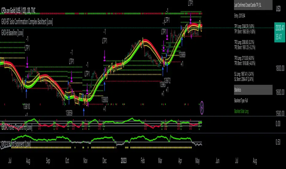
GKD-BT Solo Confirmation Simple Backtest [Loxx]Giga Kaleidoscope GKD-BT Solo Confirmation Simple Backtest is a Backtesting module included in Loxx's "Giga Kaleidoscope Modularized Trading System".
█ GKD-BT Solo Confirmation Simple Backtest
The Solo Confirmation Simple Backtest module enables users to perform Standard Long and Short signals on GKD-C confirmation indicators. This module represents the simplest form of Backtest in the GKD trading system. It includes two types of backtests: Trading and Full. The Trading backtest allows users to test individual trades, both long and short, one at a time. On the other hand, the Full backtest allows users to test either longs or shorts by toggling between them in the settings to view the results for each signal type. The Trading backtest simulates real trading, while the Full backtest tests all signals, whether long or short.
Additionally, this backtest module provides the option to test the GKD-C indicator with 1 to 3 take profits and 1 stop loss. The Trading backtest allows for the use of 1 to 3 take profits, while the Full backtest is limited to 1 take profit. The Trading backtest also offers the capability to apply a trailing take profit.
In terms of the percentage of trade removed at each take profit, this backtest module has the following hardcoded values:
Take profit 1: 50% of the trade is removed
Take profit 2: 25% of the trade is removed
Take profit 3: 25% of the trade is removed
Stop loss: 100% of the trade is removed
After each take profit is achieved, the stop loss level is adjusted. When take profit 1 is reached, the stop loss is moved to the entry point. Similarly, when take profit 2 is reached, the stop loss is shifted to take profit 1. The trailing take profit feature comes into play after take profit 2 or take profit 3, depending on the number of take profits selected in the settings. The trailing take profit is always activated on the final take profit when 2 or more take profits are chosen.
The backtest also offers the capability to restrict by a specific date range, allowing for simulated forward testing based on past data. Additionally, users have the option to display or hide a trading panel that provides relevant information about the backtest, statistics, and the current trade. It is also possible to activate alerts and toggle sections of the trading panel on or off. On the chart, historical take profit and stop loss levels are represented by horizontal lines overlaid for reference.
The GKD system utilizes volatility-based take profits and stop losses. Each take profit and stop loss is calculated as a multiple of volatility. You can change the values of the multipliers in the settings as well.
To utilize this strategy, follow these steps:
1. Adjust the "Confirmation Type" in the GKD-C Confirmation Indicator to "GKD New."
2. Import the value "Input into NEW GKD-BT Backtest" into the GKD-BT Solo Confirmation Simple Backtest module (this strategy backtest).
**The GKD-BT Solo Confirmation Simple Backtest module exclusively supports Standard Entries, both Long and Short. However, please note that this module uses a modified version of the standard entry, where long and short signals are directly imported from the Confirmation indicator without any baseline or volatility filtering applied.**
Volatility Types Included
17 types of volatility are included in this indicator
Close-to-Close
Parkinson
Garman-Klass
Rogers-Satchell
Yang-Zhang
Garman-Klass-Yang-Zhang
Exponential Weighted Moving Average
Standard Deviation of Log Returns
Pseudo GARCH(2,2)
Average True Range
True Range Double
Standard Deviation
Adaptive Deviation
Median Absolute Deviation
Efficiency-Ratio Adaptive ATR
Mean Absolute Deviation
Static Percent
Close-to-Close
Close-to-Close volatility is a classic and widely used volatility measure, sometimes referred to as historical volatility.
Volatility is an indicator of the speed of a stock price change. A stock with high volatility is one where the price changes rapidly and with a larger amplitude. The more volatile a stock is, the riskier it is.
Close-to-close historical volatility is calculated using only a stock's closing prices. It is the simplest volatility estimator. However, in many cases, it is not precise enough. Stock prices could jump significantly during a trading session and return to the opening value at the end. That means that a considerable amount of price information is not taken into account by close-to-close volatility.
Despite its drawbacks, Close-to-Close volatility is still useful in cases where the instrument doesn't have intraday prices. For example, mutual funds calculate their net asset values daily or weekly, and thus their prices are not suitable for more sophisticated volatility estimators.
Parkinson
Parkinson volatility is a volatility measure that uses the stock’s high and low price of the day.
The main difference between regular volatility and Parkinson volatility is that the latter uses high and low prices for a day, rather than only the closing price. This is useful as close-to-close prices could show little difference while large price movements could have occurred during the day. Thus, Parkinson's volatility is considered more precise and requires less data for calculation than close-to-close volatility.
One drawback of this estimator is that it doesn't take into account price movements after the market closes. Hence, it systematically undervalues volatility. This drawback is addressed in the Garman-Klass volatility estimator.
Garman-Klass
Garman-Klass is a volatility estimator that incorporates open, low, high, and close prices of a security.
Garman-Klass volatility extends Parkinson's volatility by taking into account the opening and closing prices. As markets are most active during the opening and closing of a trading session, it makes volatility estimation more accurate.
Garman and Klass also assumed that the process of price change follows a continuous diffusion process (Geometric Brownian motion). However, this assumption has several drawbacks. The method is not robust for opening jumps in price and trend movements.
Despite its drawbacks, the Garman-Klass estimator is still more effective than the basic formula since it takes into account not only the price at the beginning and end of the time interval but also intraday price extremes.
Researchers Rogers and Satchell have proposed a more efficient method for assessing historical volatility that takes into account price trends. See Rogers-Satchell Volatility for more detail.
Rogers-Satchell
Rogers-Satchell is an estimator for measuring the volatility of securities with an average return not equal to zero.
Unlike Parkinson and Garman-Klass estimators, Rogers-Satchell incorporates a drift term (mean return not equal to zero). As a result, it provides better volatility estimation when the underlying is trending.
The main disadvantage of this method is that it does not take into account price movements between trading sessions. This leads to an underestimation of volatility since price jumps periodically occur in the market precisely at the moments between sessions.
A more comprehensive estimator that also considers the gaps between sessions was developed based on the Rogers-Satchel formula in the 2000s by Yang-Zhang. See Yang Zhang Volatility for more detail.
Yang-Zhang
Yang Zhang is a historical volatility estimator that handles both opening jumps and the drift and has a minimum estimation error.
Yang-Zhang volatility can be thought of as a combination of the overnight (close-to-open volatility) and a weighted average of the Rogers-Satchell volatility and the day’s open-to-close volatility. It is considered to be 14 times more efficient than the close-to-close estimator.
Garman-Klass-Yang-Zhang
Garman-Klass-Yang-Zhang (GKYZ) volatility estimator incorporates the returns of open, high, low, and closing prices in its calculation.
GKYZ volatility estimator takes into account overnight jumps but not the trend, i.e., it assumes that the underlying asset follows a Geometric Brownian Motion (GBM) process with zero drift. Therefore, the GKYZ volatility estimator tends to overestimate the volatility when the drift is different from zero. However, for a GBM process, this estimator is eight times more efficient than the close-to-close volatility estimator.
Exponential Weighted Moving Average
The Exponentially Weighted Moving Average (EWMA) is a quantitative or statistical measure used to model or describe a time series. The EWMA is widely used in finance, with the main applications being technical analysis and volatility modeling.
The moving average is designed such that older observations are given lower weights. The weights decrease exponentially as the data point gets older – hence the name exponentially weighted.
The only decision a user of the EWMA must make is the parameter lambda. The parameter decides how important the current observation is in the calculation of the EWMA. The higher the value of lambda, the more closely the EWMA tracks the original time series.
Standard Deviation of Log Returns
This is the simplest calculation of volatility. It's the standard deviation of ln(close/close(1)).
Pseudo GARCH(2,2)
This is calculated using a short- and long-run mean of variance multiplied by ?.
?avg(var;M) + (1 ? ?) avg(var;N) = 2?var/(M+1-(M-1)L) + 2(1-?)var/(M+1-(M-1)L)
Solving for ? can be done by minimizing the mean squared error of estimation; that is, regressing L^-1var - avg(var; N) against avg(var; M) - avg(var; N) and using the resulting beta estimate as ?.
Average True Range
The average true range (ATR) is a technical analysis indicator, introduced by market technician J. Welles Wilder Jr. in his book New Concepts in Technical Trading Systems, that measures market volatility by decomposing the entire range of an asset price for that period.
The true range indicator is taken as the greatest of the following: current high less the current low; the absolute value of the current high less the previous close; and the absolute value of the current low less the previous close. The ATR is then a moving average, generally using 14 days, of the true ranges.
True Range Double
A special case of ATR that attempts to correct for volatility skew.
Standard Deviation
Standard deviation is a statistic that measures the dispersion of a dataset relative to its mean and is calculated as the square root of the variance. The standard deviation is calculated as the square root of variance by determining each data point's deviation relative to the mean. If the data points are further from the mean, there is a higher deviation within the data set; thus, the more spread out the data, the higher the standard deviation.
Adaptive Deviation
By definition, the Standard Deviation (STD, also represented by the Greek letter sigma ? or the Latin letter s) is a measure that is used to quantify the amount of variation or dispersion of a set of data values. In technical analysis, we usually use it to measure the level of current volatility.
Standard Deviation is based on Simple Moving Average calculation for mean value. This version of standard deviation uses the properties of EMA to calculate what can be called a new type of deviation, and since it is based on EMA, we can call it EMA deviation. Additionally, Perry Kaufman's efficiency ratio is used to make it adaptive (since all EMA type calculations are nearly perfect for adapting).
The difference when compared to the standard is significant--not just because of EMA usage, but the efficiency ratio makes it a "bit more logical" in very volatile market conditions.
Median Absolute Deviation
The median absolute deviation is a measure of statistical dispersion. Moreover, the MAD is a robust statistic, being more resilient to outliers in a data set than the standard deviation. In the standard deviation, the distances from the mean are squared, so large deviations are weighted more heavily, and thus outliers can heavily influence it. In the MAD, the deviations of a small number of outliers are irrelevant.
Because the MAD is a more robust estimator of scale than the sample variance or standard deviation, it works better with distributions without a mean or variance, such as the Cauchy distribution.
Efficiency-Ratio Adaptive ATR
Average True Range (ATR) is a widely used indicator for many occasions in technical analysis. It is calculated as the RMA of the true range. This version adds a "twist": it uses Perry Kaufman's Efficiency Ratio to calculate adaptive true range.
Mean Absolute Deviation
The mean absolute deviation (MAD) is a measure of variability that indicates the average distance between observations and their mean. MAD uses the original units of the data, which simplifies interpretation. Larger values signify that the data points spread out further from the average. Conversely, lower values correspond to data points bunching closer to it. The mean absolute deviation is also known as the mean deviation and average absolute deviation.
This definition of the mean absolute deviation sounds similar to the standard deviation (SD). While both measure variability, they have different calculations. In recent years, some proponents of MAD have suggested that it replace the SD as the primary measure because it is a simpler concept that better fits real life.
Static Percent
Static Percent allows the user to insert their own constant percent that will then be used to create take profits and stoploss
█ Giga Kaleidoscope Modularized Trading System
Core components of an NNFX algorithmic trading strategy
The NNFX algorithm is built on the principles of trend, momentum, and volatility. There are six core components in the NNFX trading algorithm:
1. Volatility - price volatility; e.g., Average True Range, True Range Double, Close-to-Close, etc.
2. Baseline - a moving average to identify price trend
3. Confirmation 1 - a technical indicator used to identify trends
4. Confirmation 2 - a technical indicator used to identify trends
5. Continuation - a technical indicator used to identify trends
6. Volatility/Volume - a technical indicator used to identify volatility/volume breakouts/breakdown
7. Exit - a technical indicator used to determine when a trend is exhausted
What is Volatility in the NNFX trading system?
In the NNFX (No Nonsense Forex) trading system, ATR (Average True Range) is typically used to measure the volatility of an asset. It is used as a part of the system to help determine the appropriate stop loss and take profit levels for a trade. ATR is calculated by taking the average of the true range values over a specified period.
True range is calculated as the maximum of the following values:
-Current high minus the current low
-Absolute value of the current high minus the previous close
-Absolute value of the current low minus the previous close
ATR is a dynamic indicator that changes with changes in volatility. As volatility increases, the value of ATR increases, and as volatility decreases, the value of ATR decreases. By using ATR in NNFX system, traders can adjust their stop loss and take profit levels according to the volatility of the asset being traded. This helps to ensure that the trade is given enough room to move, while also minimizing potential losses.
Other types of volatility include True Range Double (TRD), Close-to-Close, and Garman-Klass
What is a Baseline indicator?
The baseline is essentially a moving average, and is used to determine the overall direction of the market.
The baseline in the NNFX system is used to filter out trades that are not in line with the long-term trend of the market. The baseline is plotted on the chart along with other indicators, such as the Moving Average (MA), the Relative Strength Index (RSI), and the Average True Range (ATR).
Trades are only taken when the price is in the same direction as the baseline. For example, if the baseline is sloping upwards, only long trades are taken, and if the baseline is sloping downwards, only short trades are taken. This approach helps to ensure that trades are in line with the overall trend of the market, and reduces the risk of entering trades that are likely to fail.
By using a baseline in the NNFX system, traders can have a clear reference point for determining the overall trend of the market, and can make more informed trading decisions. The baseline helps to filter out noise and false signals, and ensures that trades are taken in the direction of the long-term trend.
What is a Confirmation indicator?
Confirmation indicators are technical indicators that are used to confirm the signals generated by primary indicators. Primary indicators are the core indicators used in the NNFX system, such as the Average True Range (ATR), the Moving Average (MA), and the Relative Strength Index (RSI).
The purpose of the confirmation indicators is to reduce false signals and improve the accuracy of the trading system. They are designed to confirm the signals generated by the primary indicators by providing additional information about the strength and direction of the trend.
Some examples of confirmation indicators that may be used in the NNFX system include the Bollinger Bands, the MACD (Moving Average Convergence Divergence), and the MACD Oscillator. These indicators can provide information about the volatility, momentum, and trend strength of the market, and can be used to confirm the signals generated by the primary indicators.
In the NNFX system, confirmation indicators are used in combination with primary indicators and other filters to create a trading system that is robust and reliable. By using multiple indicators to confirm trading signals, the system aims to reduce the risk of false signals and improve the overall profitability of the trades.
What is a Continuation indicator?
In the NNFX (No Nonsense Forex) trading system, a continuation indicator is a technical indicator that is used to confirm a current trend and predict that the trend is likely to continue in the same direction. A continuation indicator is typically used in conjunction with other indicators in the system, such as a baseline indicator, to provide a comprehensive trading strategy.
What is a Volatility/Volume indicator?
Volume indicators, such as the On Balance Volume (OBV), the Chaikin Money Flow (CMF), or the Volume Price Trend (VPT), are used to measure the amount of buying and selling activity in a market. They are based on the trading volume of the market, and can provide information about the strength of the trend. In the NNFX system, volume indicators are used to confirm trading signals generated by the Moving Average and the Relative Strength Index. Volatility indicators include Average Direction Index, Waddah Attar, and Volatility Ratio. In the NNFX trading system, volatility is a proxy for volume and vice versa.
By using volume indicators as confirmation tools, the NNFX trading system aims to reduce the risk of false signals and improve the overall profitability of trades. These indicators can provide additional information about the market that is not captured by the primary indicators, and can help traders to make more informed trading decisions. In addition, volume indicators can be used to identify potential changes in market trends and to confirm the strength of price movements.
What is an Exit indicator?
The exit indicator is used in conjunction with other indicators in the system, such as the Moving Average (MA), the Relative Strength Index (RSI), and the Average True Range (ATR), to provide a comprehensive trading strategy.
The exit indicator in the NNFX system can be any technical indicator that is deemed effective at identifying optimal exit points. Examples of exit indicators that are commonly used include the Parabolic SAR, the Average Directional Index (ADX), and the Chandelier Exit.
The purpose of the exit indicator is to identify when a trend is likely to reverse or when the market conditions have changed, signaling the need to exit a trade. By using an exit indicator, traders can manage their risk and prevent significant losses.
In the NNFX system, the exit indicator is used in conjunction with a stop loss and a take profit order to maximize profits and minimize losses. The stop loss order is used to limit the amount of loss that can be incurred if the trade goes against the trader, while the take profit order is used to lock in profits when the trade is moving in the trader's favor.
Overall, the use of an exit indicator in the NNFX trading system is an important component of a comprehensive trading strategy. It allows traders to manage their risk effectively and improve the profitability of their trades by exiting at the right time.
How does Loxx's GKD (Giga Kaleidoscope Modularized Trading System) implement the NNFX algorithm outlined above?
Loxx's GKD v2.0 system has five types of modules (indicators/strategies). These modules are:
1. GKD-BT - Backtesting module (Volatility, Number 1 in the NNFX algorithm)
2. GKD-B - Baseline module (Baseline and Volatility/Volume, Numbers 1 and 2 in the NNFX algorithm)
3. GKD-C - Confirmation 1/2 and Continuation module (Confirmation 1/2 and Continuation, Numbers 3, 4, and 5 in the NNFX algorithm)
4. GKD-V - Volatility/Volume module (Confirmation 1/2, Number 6 in the NNFX algorithm)
5. GKD-E - Exit module (Exit, Number 7 in the NNFX algorithm)
(additional module types will added in future releases)
Each module interacts with every module by passing data to A backtest module wherein the various components of the GKD system are combined to create a trading signal.
That is, the Baseline indicator passes its data to Volatility/Volume. The Volatility/Volume indicator passes its values to the Confirmation 1 indicator. The Confirmation 1 indicator passes its values to the Confirmation 2 indicator. The Confirmation 2 indicator passes its values to the Continuation indicator. The Continuation indicator passes its values to the Exit indicator, and finally, the Exit indicator passes its values to the Backtest strategy.
This chaining of indicators requires that each module conform to Loxx's GKD protocol, therefore allowing for the testing of every possible combination of technical indicators that make up the six components of the NNFX algorithm.
What does the application of the GKD trading system look like?
Example trading system:
Backtest: Solo Confirmation Simple Backtest as shown on the chart above
Baseline: Hull Moving Average
Volatility/Volume: Hurst Exponent
Confirmation 1: Fisher Trasnform as shown on the chart above
Confirmation 2: Williams Percent Range
Continuation: Volatility-Adaptive Rapid RSI T3
Exit: Rex Oscillator
Each GKD indicator is denoted with a module identifier of either: GKD-BT, GKD-B, GKD-C, GKD-V, or GKD-E. This allows traders to understand to which module each indicator belongs and where each indicator fits into the GKD system.
Giga Kaleidoscope Modularized Trading System Signals (based on the NNFX algorithm)
Standard Entry
1. GKD-C Confirmation 1 Signal
2. GKD-B Baseline agrees
3. Price is within a range of 0.2x Volatility and 1.0x Volatility of the Goldie Locks Mean
4. GKD-C Confirmation 2 agrees
5. GKD-V Volatility/Volume agrees
Baseline Entry
1. GKD-B Baseline signal
2. GKD-C Confirmation 1 agrees
3. Price is within a range of 0.2x Volatility and 1.0x Volatility of the Goldie Locks Mean
4. GKD-C Confirmation 2 agrees
5. GKD-V Volatility/Volume agrees
6. GKD-C Confirmation 1 signal was less than 7 candles prior
Volatility/Volume Entry
1. GKD-V Volatility/Volume signal
2. GKD-C Confirmation 1 agrees
3. Price is within a range of 0.2x Volatility and 1.0x Volatility of the Goldie Locks Mean
4. GKD-C Confirmation 2 agrees
5. GKD-B Baseline agrees
6. GKD-C Confirmation 1 signal was less than 7 candles prior
Continuation Entry
1. Standard Entry, Baseline Entry, or Pullback; entry triggered previously
2. GKD-B Baseline hasn't crossed since entry signal trigger
3. GKD-C Confirmation Continuation Indicator signals
4. GKD-C Confirmation 1 agrees
5. GKD-B Baseline agrees
6. GKD-C Confirmation 2 agrees
1-Candle Rule Standard Entry
1. GKD-C Confirmation 1 signal
2. GKD-B Baseline agrees
3. Price is within a range of 0.2x Volatility and 1.0x Volatility of the Goldie Locks Mean
Next Candle:
1. Price retraced (Long: close < close or Short: close > close )
2. GKD-B Baseline agrees
3. GKD-C Confirmation 1 agrees
4. GKD-C Confirmation 2 agrees
5. GKD-V Volatility/Volume agrees
1-Candle Rule Baseline Entry
1. GKD-B Baseline signal
2. GKD-C Confirmation 1 agrees
3. Price is within a range of 0.2x Volatility and 1.0x Volatility of the Goldie Locks Mean
4. GKD-C Confirmation 1 signal was less than 7 candles prior
Next Candle:
1. Price retraced (Long: close < close or Short: close > close )
2. GKD-B Baseline agrees
3. GKD-C Confirmation 1 agrees
4. GKD-C Confirmation 2 agrees
5. GKD-V Volatility/Volume Agrees
1-Candle Rule Volatility/Volume Entry
1. GKD-V Volatility/Volume signal
2. GKD-C Confirmation 1 agrees
3. Price is within a range of 0.2x Volatility and 1.0x Volatility of the Goldie Locks Mean
4. GKD-C Confirmation 1 signal was less than 7 candles prior
Next Candle:
1. Price retraced (Long: close < close or Short: close > close)
2. GKD-B Volatility/Volume agrees
3. GKD-C Confirmation 1 agrees
4. GKD-C Confirmation 2 agrees
5. GKD-B Baseline agrees
PullBack Entry
1. GKD-B Baseline signal
2. GKD-C Confirmation 1 agrees
3. Price is beyond 1.0x Volatility of Baseline
Next Candle:
1. Price is within a range of 0.2x Volatility and 1.0x Volatility of the Goldie Locks Mean
2. GKD-C Confirmation 1 agrees
3. GKD-C Confirmation 2 agrees
4. GKD-V Volatility/Volume Agrees
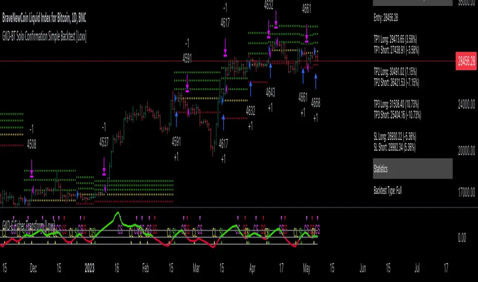
Daily Dax Strategy
-----------------
Hey there!
There are a lot of reasons why this strategy has performed very well in recent years.
A very simple strategy in itself. The system basically follows the trend following approach. The focus is always on rising trends. No action takes place during falling trends. Both time filters and trend filters are used. There is only one position per day which is compulsorily closed again at the end of the time filter.
Only for CURRENCYCOM:DE30 !
The indicator is designed for the h1 hourly chart. In addition, the display can be adjusted using the options.
That's all. Due to the economic background, the strategy can be used without a large technical chart analysis.
Warning: Before contacting a position, it is always more important than having strong news. Better to play it safe in these same ones.
Caution: With this strategy, as an exception, no SL is allowed by default. Therefore always calculate the risk carefully.
Past results do not guarantee future profits!
Follow the link below to get access to this indicator or get us a PM to get access.
--------------------------------------------------------------------------------------------------------------
--------------------------------------------------------------------------------------------------------------
-----------------
Willkommen!
Es gibt viele Gründe, warum sich diese Strategie in den letzten Jahren ganz gut bewährt hat.
Eine sehr einfache Strategie für sich. Grundsätzlich folgt das System dem Trendfolge Ansatz. Es wird immer nur auf steigende Trends gesetzt. Während fallenden Trends finden keine Aktionen statt. Es werden sowohl Zeitfilter als auch Trendfilter verwendet. Es gibt nur eine Position am Tag welche zwingend auch am Ende des Zeitfilters wieder geschlossen wird.
Only for CURRENCYCOM:DE30 !
Der Indikator ist für den h1 Stundechart ausgelegt. Zusätzlich kann die Anzeige über die Optionen angepasst werden.
Das ist alles. Aufgrund des wirtschaftlichen Hintergrunds kann die Strategie ohne umfangreiche technische Chartanalyse verwendet werden.
Achtung: Vor dem Öffnen einer Positionen immer zuerst prüfen ob starke News anstehen. In diesen Fällen lieber auf Nummer sicher gehen.
Achtung: Bei dieser Strategie ist standardmäßig ausnahmsweise kein SL vorgesehen. Daher das Risiko Immer gut kalkulieren.
Vergangene Ergebnisse garantieren keine zukünftigen Gewinne!
Verwenden Sie den folgenden Link, um Zugriff auf diesen Indikator zu erhalten oder schreibe uns eine PM um Zugriff zu erhalten.

1 Triple EMA Crossover Strategy (x, 3x, 9x)An excellent EMA strategy.
x, 3x, and 9x: These represent the periods of the EMAs. For example, if 'x' is 10, then you would have a 10-day EMA, a 30-day EMA, and a 90-day EMA.
Crossover: The strategy relies on identifying when the price or the shorter-term EMAs cross above or below the longer-term EMAs, signaling potential buy or sell opportunities.
How the Strategy Works:
1. Trend Identification:
The relationship between the three EMAs indicates the overall trend. If the 3x EMA is above the 9x EMA, and the x EMA is above both, it suggests an uptrend. Conversely, if the 3x EMA is below the 9x EMA, and the x EMA is below both, it indicates a downtrend.
2. Buy Signals:
A buy signal might be generated when the shortest EMA (x) crosses above the medium EMA (3x) and then both cross above the longest EMA (9x), suggesting a potential breakout.
3. Sell Signals:
A sell signal might be generated when the shortest EMA (x) crosses below the medium EMA (3x) and then both cross below the longest EMA (9x), suggesting a potential breakdown.
---------------------------------------------------------------------------------------------------------
Unlocking Trends with the Triple EMA Crossover Strategy (x, 3x, 9x)
Welcome to an intuitive yet powerful trend-following strategy designed for clarity and actionable signals: the Triple EMA Crossover. This Pine Script® indicator leverages the Exponential Moving Average (EMA) to help traders identify prevailing trends, potential breakouts, and breakdowns with enhanced precision. Built on a simple, scalable 'x, 3x, 9x' methodology, it provides a dynamic framework for navigating market movements.
Understanding the x, 3x, 9x EMA Foundation
At its core, this strategy utilizes three Exponential Moving Averages, each acting as a distinct lens on price action. Unlike Simple Moving Averages (SMAs) which give equal weight to all data points, EMAs place a greater emphasis on recent prices, making them more responsive to current market conditions—a crucial advantage in fast-paced environments like intraday trading.
The "x, 3x, 9x" nomenclature is elegantly simple:
x EMA (Fast EMA): This is your shortest-period EMA, highly sensitive to immediate price changes. It acts as the leading indicator, quickly reacting to shifts in momentum.
3x EMA (Medium EMA): Calculated with three times the 'x' period, this EMA provides a smoother, yet still responsive, view of the short-to-medium term trend. It often acts as dynamic support or resistance.
9x EMA (Slow EMA): Representing nine times the 'x' period, this is your longest EMA. It filters out much of the market noise, giving you a clear picture of the underlying dominant trend.
The beauty of this setup lies in its adaptability. By simply adjusting the Base EMA Period (x) input in the script settings, you can automatically calibrate all three EMAs to suit different instruments, volatility levels, or even your preferred trading style. A common starting point for 'x' in intraday trading on a 5-minute chart is 10, which translates to 10, 30, and 90-period EMAs.
How the Strategy Works: Signals and Trend Identification
The power of the Triple EMA Crossover lies in the interplay and alignment of these three moving averages.
1. Trend Identification
The relative positioning of the EMAs paints a clear picture of the market's trend:
Uptrend (Bullish): When the emaX (fast) is above the ema3X (medium), and the ema3X is, in turn, above the ema9X (slow), it indicates a strong bullish trend. This "stacked" alignment suggests robust upward momentum.
Downtrend (Bearish): Conversely, if the emaX (fast) is below the ema3X (medium), and the ema3X is below the ema9X (slow), it signals a clear bearish trend.
2. Buy Signals 🟢
A buy signal is generated when the swift emaX crosses above the ema3X, AND simultaneously, the ema3X is already above the ema9X. This combined condition ensures that the shorter-term momentum is shifting upward while the underlying medium-term trend remains strong and aligned with the longer-term direction. This reduces false signals often seen with simple two-EMA crossovers, aiming to capture high-probability upward moves. The script will plot a green upward-pointing triangle below the candle to visually alert you to this entry.
3. Sell Signals 🔴
A sell signal occurs when the quick emaX crosses below the ema3X, AND the ema3X is already below the ema9X. This indicates that the short-term momentum is shifting downwards, confirming a bearish bias within the broader downtrend. This comprehensive confirmation helps identify potential breakdowns and exit points for long positions or entry points for short trades. A red downward-pointing triangle will appear above the candle to mark this signal.
The strategy also includes an intuitive exit mechanism: if a buy signal is active and a sell condition is met, the long position will be closed, and vice-versa for short positions. This ensures you're always aligned with the most recent confirmed trend direction.
Key Advantages for Traders
Clarity: Provides visually clear trend direction and momentum shifts.
Responsiveness: EMAs react faster to price changes compared to SMAs, making them ideal for dynamic markets.
Confirmation: The three-EMA alignment significantly reduces false signals, leading to higher-conviction trades.
Adaptability: The x input allows you to fine-tune the strategy for various assets and market conditions.
Simplicity: Despite its effectiveness, the logic remains straightforward and easy to understand.
Important Considerations for Day Trading
For optimal performance in intraday trading, it's highly recommended to apply this strategy on a 5-minute chart. This timeframe strikes the perfect balance between capturing rapid price action and filtering out excessive market noise, allowing the EMA crossovers to provide meaningful signals. Always combine this technical analysis with sound risk management, including stop-loss orders, and consider other indicators or fundamental analysis for further confirmation.
Customization and Disclaimer
Feel free to experiment with the Base EMA Period (x) input to find the optimal settings that resonate with your trading style and the specific instruments you trade. Remember, no single strategy guarantees profits, and past performance is not indicative of future results. This script is provided for educational and illustrative purposes. Always conduct your own research and risk assessment before trading with real capital. Happy Trading!
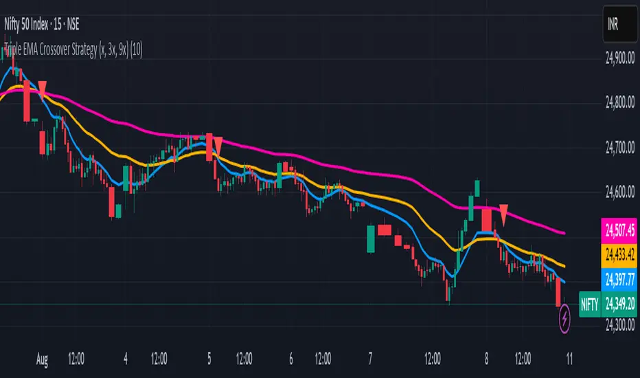
Fusion Sniper X [ Crypto Strategy]📌 Fusion Sniper X — Description for TradingView
Overview:
Fusion Sniper X is a purpose-built algorithmic trading strategy designed for cryptocurrency markets, especially effective on the 1-hour chart. It combines advanced trend analysis, momentum filtering, volatility confirmation, and dynamic trade management to deliver a fast-reacting, high-precision trading system. This script is not a basic mashup of indicators, but a fully integrated strategy with logical synergy between components, internal equity management, and visual trade analytics via a customizable dashboard.
🔍 How It Works
🔸 Trend Detection – McGinley Dynamic + Gradient Slope
McGinley Dynamic is used as the baseline to reflect adaptive price action more responsively than standard moving averages.
A custom gradient filter, calculated using the slope of the McGinley line normalized by ATR, determines if the market is trending up or down.
trendUp when slope > 0
trendDown when slope < 0
🔸 Momentum Confirmation – ZLEMA-Smoothed CCI
CCI (Commodity Channel Index) is used to detect momentum strength and direction.
It is further smoothed with ZLEMA (Zero Lag EMA) to reduce noise while keeping lag minimal.
Entry is confirmed when:
CCI > 0 (Bullish momentum)
CCI < 0 (Bearish momentum)
🔸 Volume Confirmation – Relative Volume Spike Filter
Uses a 20-period EMA of volume to calculate the expected average.
Trades are only triggered if real-time volume exceeds this average by a user-defined multiplier (default: 1.5x), filtering out low-conviction signals.
🔸 Trap Detection – Wick-to-Body Reversal Filter
Filters out potential trap candles using wick-to-body ratio and body size compared to ATR.
Avoids entering on manipulative price spikes where:
Long traps show large lower wicks.
Short traps show large upper wicks.
🔸 Entry Conditions
A trade is only allowed when:
Within selected date range
Cooldown between trades is respected
Daily drawdown guard is not triggered
All of the following align:
Trend direction (McGinley slope)
Momentum confirmation (CCI ZLEMA)
Volume spike active
No trap candle detected
🎯 Trade Management Logic
✅ Take Profit (TP1/TP2 System)
TP1: 50% of the position is closed at a predefined % gain (default 2%).
TP2: Remaining 100% is closed at a higher profit level (default 4%).
🛑 Stop Loss
A fixed 2% stop loss is enforced per position using strategy.exit(..., stop=...) logic.
Stop loss is active for both TP2 and primary entries and updates the dashboard if triggered.
❄️ Cooldown & Equity Protection
A user-defined cooldown period (in bars) prevents overtrading.
A daily equity loss guard blocks new trades if portfolio drawdown exceeds a % threshold (default: 2.5%).
📊 Real-Time Dashboard (On-Chart Table)
Fusion Sniper X features a futuristic, color-coded dashboard with theme controls, showing:
Current position and entry price
Real-time profit/loss (%)
TP1, TP2, and SL status
Trend and momentum direction
Volume spike state and trap candle alerts
Trade statistics: total, win/loss, drawdown
Symbol and timeframe display
Themes include: Neon, Cyber, Monochrome, and Dark Techno.
📈 Visuals
McGinley baseline is plotted in orange for trend bias.
Bar colors reflect active positions (green for long, red for short).
Stop loss line plotted in red when active.
Background shading highlights active volume spikes.
✅ Why It’s Not Just a Mashup
Fusion Sniper X is an original system architecture built on:
Custom logic (gradient-based trend slope, wick trap rejection)
Synergistic indicator stacking (ZLEMA-smoothed momentum, ATR-based slope)
Position and equity tracking (not just signal-based plotting)
Intelligent risk control with take-profits, stop losses, cooldown, and max loss rules
An interactive dashboard that enhances usability and transparency
Every component has a distinct role in the system, and none are used as-is from public sources without modification or integration logic. The design follows a cohesive and rule-based structure for algorithmic execution.
⚠️ Disclaimer
This strategy is for educational and informational purposes only. It does not constitute financial advice. Trading cryptocurrencies involves substantial risk, and past performance is not indicative of future results. Always backtest and forward-test before using on a live account. Use at your own risk.
📅 Backtest Range & Market Conditions Note
The performance results displayed for Fusion Sniper X are based on a focused backtest period from December 1, 2024 to May 10, 2025. This range was chosen intentionally due to the dynamic and volatile nature of cryptocurrency markets, where structural and behavioral shifts can occur rapidly. By evaluating over a shorter, recent time window, the strategy is tuned to current market mechanics and avoids misleading results that could come from outdated market regimes. This ensures more realistic, forward-aligned performance — particularly important for high-frequency systems operating on the 1-hour timeframe.

Multi-Step FlexiSuperTrend - Strategy [presentTrading]At the heart of this endeavor is a passion for continuous improvement in the art of trading
█ Introduction and How it is Different
The "Multi-Step FlexiSuperTrend - Strategy " is an advanced trading strategy that integrates the well-known SuperTrend indicator with a nuanced and dynamic approach to market trend analysis. Unlike conventional SuperTrend strategies that rely on static thresholds and fixed parameters, this strategy introduces multi-step take profit mechanisms that allow traders to capitalize on varying market conditions in a more controlled and systematic manner.
What sets this strategy apart is its ability to dynamically adjust to market volatility through the use of an incremental factor applied to the SuperTrend calculation. This adjustment ensures that the strategy remains responsive to both minor and major market shifts, providing a more accurate signal for entries and exits. Additionally, the integration of multi-step take profit levels offers traders the flexibility to scale out of positions, locking in profits progressively as the market moves in their favor.
BTC 6hr Long/Short Performance
█ Strategy, How it Works: Detailed Explanation
The Multi-Step FlexiSuperTrend strategy operates on the foundation of the SuperTrend indicator, but with several enhancements that make it more adaptable to varying market conditions. The key components of this strategy include the SuperTrend Polyfactor Oscillator, a dynamic normalization process, and multi-step take profit levels.
🔶 SuperTrend Polyfactor Oscillator
The SuperTrend Polyfactor Oscillator is the heart of this strategy. It is calculated by applying a series of SuperTrend calculations with varying factors, starting from a defined "Starting Factor" and incrementing by a specified "Increment Factor." The indicator length and the chosen price source (e.g., HLC3, HL2) are inputs to the oscillator.
The SuperTrend formula typically calculates an upper and lower band based on the average true range (ATR) and a multiplier (the factor). These bands determine the trend direction. In the FlexiSuperTrend strategy, the oscillator is enhanced by iteratively applying the SuperTrend calculation across different factors. The iterative process allows the strategy to capture both minor and significant trend changes.
For each iteration (indexed by `i`), the following calculations are performed:
1. ATR Calculation: The Average True Range (ATR) is calculated over the specified `indicatorLength`:
ATR_i = ATR(indicatorLength)
2. Upper and Lower Bands Calculation: The upper and lower bands are calculated using the ATR and the current factor:
Upper Band_i = hl2 + (ATR_i * Factor_i)
Lower Band_i = hl2 - (ATR_i * Factor_i)
Here, `Factor_i` starts from `startingFactor` and is incremented by `incrementFactor` in each iteration.
3. Trend Determination: The trend is determined by comparing the indicator source with the upper and lower bands:
Trend_i = 1 (uptrend) if IndicatorSource > Upper Band_i
Trend_i = 0 (downtrend) if IndicatorSource < Lower Band_i
Otherwise, the trend remains unchanged from the previous value.
4. Output Calculation: The output of each iteration is determined based on the trend:
Output_i = Lower Band_i if Trend_i = 1
Output_i = Upper Band_i if Trend_i = 0
This process is repeated for each iteration (from 0 to 19), creating a series of outputs that reflect different levels of trend sensitivity.
Local
🔶 Normalization Process
To make the oscillator values comparable across different market conditions, the deviations between the indicator source and the SuperTrend outputs are normalized. The normalization method can be one of the following:
1. Max-Min Normalization: The deviations are normalized based on the range of the deviations:
Normalized Value_i = (Deviation_i - Min Deviation) / (Max Deviation - Min Deviation)
2. Absolute Sum Normalization: The deviations are normalized based on the sum of absolute deviations:
Normalized Value_i = Deviation_i / Sum of Absolute Deviations
This normalization ensures that the oscillator values are within a consistent range, facilitating more reliable trend analysis.
For more details:
🔶 Multi-Step Take Profit Mechanism
One of the unique features of this strategy is the multi-step take profit mechanism. This allows traders to lock in profits at multiple levels as the market moves in their favor. The strategy uses three take profit levels, each defined as a percentage increase (for long trades) or decrease (for short trades) from the entry price.
1. First Take Profit Level: Calculated as a percentage increase/decrease from the entry price:
TP_Level1 = Entry Price * (1 + tp_level1 / 100) for long trades
TP_Level1 = Entry Price * (1 - tp_level1 / 100) for short trades
The strategy exits a portion of the position (defined by `tp_percent1`) when this level is reached.
2. Second Take Profit Level: Similar to the first level, but with a higher percentage:
TP_Level2 = Entry Price * (1 + tp_level2 / 100) for long trades
TP_Level2 = Entry Price * (1 - tp_level2 / 100) for short trades
The strategy exits another portion of the position (`tp_percent2`) at this level.
3. Third Take Profit Level: The final take profit level:
TP_Level3 = Entry Price * (1 + tp_level3 / 100) for long trades
TP_Level3 = Entry Price * (1 - tp_level3 / 100) for short trades
The remaining portion of the position (`tp_percent3`) is exited at this level.
This multi-step approach provides a balance between securing profits and allowing the remaining position to benefit from continued favorable market movement.
█ Trade Direction
The strategy allows traders to specify the trade direction through the `tradeDirection` input. The options are:
1. Both: The strategy will take both long and short positions based on the entry signals.
2. Long: The strategy will only take long positions.
3. Short: The strategy will only take short positions.
This flexibility enables traders to tailor the strategy to their market outlook or current trend analysis.
█ Usage
To use the Multi-Step FlexiSuperTrend strategy, traders need to set the input parameters according to their trading style and market conditions. The strategy is designed for versatility, allowing for various market environments, including trending and ranging markets.
Traders can also adjust the multi-step take profit levels and percentages to match their risk management and profit-taking preferences. For example, in highly volatile markets, traders might set wider take profit levels with smaller percentages at each level to capture larger price movements.
The normalization method and the incremental factor can be fine-tuned to adjust the sensitivity of the SuperTrend Polyfactor Oscillator, making the strategy more responsive to minor market shifts or more focused on significant trends.
█ Default Settings
The default settings of the strategy are carefully chosen to provide a balanced approach between risk management and profit potential. Here is a breakdown of the default settings and their effects on performance:
1. Indicator Length (10): This parameter controls the lookback period for the ATR calculation. A shorter length makes the strategy more sensitive to recent price movements, potentially generating more signals. A longer length smooths out the ATR, reducing sensitivity but filtering out noise.
2. Starting Factor (0.618): This is the initial multiplier used in the SuperTrend calculation. A lower starting factor makes the SuperTrend bands closer to the price, generating more frequent trend changes. A higher starting factor places the bands further away, filtering out minor fluctuations.
3. Increment Factor (0.382): This parameter controls how much the factor increases with each iteration of the SuperTrend calculation. A smaller increment factor results in more gradual changes in sensitivity, while a larger increment factor creates a wider range of sensitivity across the iterations.
4. Normalization Method (None): The default is no normalization, meaning the raw deviations are used. Normalization methods like Max-Min or Absolute Sum can make the deviations more consistent across different market conditions, improving the reliability of the oscillator.
5. Take Profit Levels (2%, 8%, 18%): These levels define the thresholds for exiting portions of the position. Lower levels (e.g., 2%) capture smaller profits quickly, while higher levels (e.g., 18%) allow positions to run longer for more significant gains.
6. Take Profit Percentages (30%, 20%, 15%): These percentages determine how much of the position is exited at each take profit level. A higher percentage at the first level locks in more profit early, reducing exposure to market reversals. Lower percentages at higher levels allow for a portion of the position to benefit from extended trends.
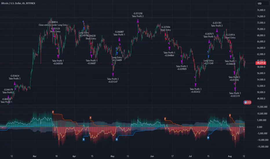
Trend Deviation strategy - BTC [IkkeOmar]Intro:
This is an example if anyone needs a push to get started with making strategies in pine script. This is an example on BTC, obviously it isn't a good strategy, and I wouldn't share my own good strategies because of alpha decay.
This strategy integrates several technical indicators to determine market trends and potential trade setups. These indicators include:
Directional Movement Index (DMI)
Bollinger Bands (BB)
Schaff Trend Cycle (STC)
Moving Average Convergence Divergence (MACD)
Momentum Indicator
Aroon Indicator
Supertrend Indicator
Relative Strength Index (RSI)
Exponential Moving Average (EMA)
Volume Weighted Average Price (VWAP)
It's crucial for you guys to understand the strengths and weaknesses of each indicator and identify synergies between them to improve the strategy's effectiveness.
Indicator Settings:
DMI (Directional Movement Index):
Length: This parameter determines the number of bars used in calculating the DMI. A higher length may provide smoother results but might lag behind the actual price action.
Bollinger Bands:
Length: This parameter specifies the number of bars used to calculate the moving average for the Bollinger Bands. A longer length results in a smoother average but might lag behind the price action.
Multiplier: The multiplier determines the width of the Bollinger Bands. It scales the standard deviation of the price data. A higher multiplier leads to wider bands, indicating increased volatility, while a lower multiplier results in narrower bands, suggesting decreased volatility.
Schaff Trend Cycle (STC):
Length: This parameter defines the length of the STC calculation. A longer length may result in smoother but slower-moving signals.
Fast Length: Specifies the length of the fast moving average component in the STC calculation.
Slow Length: Specifies the length of the slow moving average component in the STC calculation.
MACD (Moving Average Convergence Divergence):
Fast Length: Determines the number of bars used to calculate the fast EMA (Exponential Moving Average) in the MACD.
Slow Length: Specifies the number of bars used to calculate the slow EMA in the MACD.
Signal Length: Defines the number of bars used to calculate the signal line, which is typically an EMA of the MACD line.
Momentum Indicator:
Length: This parameter sets the number of bars over which momentum is calculated. A longer length may provide smoother momentum readings but might lag behind significant price changes.
Aroon Indicator:
Length: Specifies the number of bars over which the Aroon indicator calculates its values. A longer length may result in smoother Aroon readings but might lag behind significant market movements.
Supertrend Indicator:
Trendline Length: Determines the length of the period used in the Supertrend calculation. A longer length results in a smoother trendline but might lag behind recent price changes.
Trendline Factor: Specifies the multiplier used in calculating the trendline. It affects the sensitivity of the indicator to price changes.
RSI (Relative Strength Index):
Length: This parameter sets the number of bars over which RSI calculates its values. A longer length may result in smoother RSI readings but might lag behind significant price changes.
EMA (Exponential Moving Average):
Fast EMA: Specifies the number of bars used to calculate the fast EMA. A shorter period results in a more responsive EMA to recent price changes.
Slow EMA: Determines the number of bars used to calculate the slow EMA. A longer period results in a smoother EMA but might lag behind recent price changes.
VWAP (Volume Weighted Average Price):
Default settings are typically used for VWAP calculations, which consider the volume traded at each price level over a specific period. This indicator provides insights into the average price weighted by trading volume.
backtest range and rules:
You can specify the start date for backtesting purposes.
You can can select the desired trade direction: Long, Short, or Both.
Entry and Exit Conditions:
LONG:
DMI Cross Up: The Directional Movement Index (DMI) indicates a bullish trend when the positive directional movement (+DI) crosses above the negative directional movement (-DI).
Bollinger Bands (BB): The price is below the upper Bollinger Band, indicating a potential reversal from the upper band.
Momentum Indicator: Momentum is positive, suggesting increasing buying pressure.
MACD (Moving Average Convergence Divergence): The MACD line is above the signal line, indicating bullish momentum.
Supertrend Indicator: The Supertrend indicator signals an uptrend.
Schaff Trend Cycle (STC): The STC indicates a bullish trend.
Aroon Indicator: The Aroon indicator signals a bullish trend or crossover.
When all these conditions are met simultaneously, the strategy considers it a favorable opportunity to enter a long trade.
SHORT:
DMI Cross Down: The Directional Movement Index (DMI) indicates a bearish trend when the negative directional movement (-DI) crosses above the positive directional movement (+DI).
Bollinger Bands (BB): The price is above the lower Bollinger Band, suggesting a potential reversal from the lower band.
Momentum Indicator: Momentum is negative, indicating increasing selling pressure.
MACD (Moving Average Convergence Divergence): The MACD line is below the signal line, signaling bearish momentum.
Supertrend Indicator: The Supertrend indicator signals a downtrend.
Schaff Trend Cycle (STC): The STC indicates a bearish trend.
Aroon Indicator: The Aroon indicator signals a bearish trend or crossover.
When all these conditions align, the strategy considers it an opportune moment to enter a short trade.
Disclaimer:
THIS ISN'T AN OPTIMAL STRATEGY AT ALL! It was just an old project from when I started learning pine script!
The backtest doesn't promise the same results in the future, always do both in-sample and out-of-sample testing when backtesting a strategy. And make sure you forward test it as well before implementing it!
Furthermore this strategy uses both trend and mean-reversion systems, that is usually a no-go if you want to build robust trend systems .
Don't hesitate to comment if you have any questions or if you have some good notes for a beginner.

Single Swing Strategy (SSS)Introduction
The Single Swing Strategy (SSS) is a trading strategy designed for assets that trend. It utilises a single technical indicator to identify potential buying opportunities in upward-trending markets. The strategy focuses on moments when the price of an asset breaks out to a new high, suggesting a strong upward momentum.
Components
1. Exponential Moving Averages (EMAs): SSS uses two EMAs to evaluate the overall asset trend. SSS describes an uptrend as identified, when the fast EMA crosses above the slow EMA and vice versa for a downtrend.
2. Breakout: The strategy validates the trend identified by the EMAs through breakouts in the price action of the asset over a specified lookback period. No indicator is required for this step.
3. Average Directional Index (ADX): The ADX is used to measure the strength of a trend. It does not indicate the trend's direction but rather its strength, whether it's an uptrend or downtrend. A high ADX value (typically above 25) suggests a strong trend, either up or down while a low ADX value (typically below 20) indicates a weak or non-trending market. The ADX itself is a moving average of the expanding range between the +DI and -DI.
4. Positive Directional Indicator (DI+): DI+ helps identify the presence and strength of uptrends. It is calculated based on the upward price movement between current and previous highs. A rising DI+ alongside a rising ADX suggests a strengthening uptrend. When DI+ crosses above DI-, it's often interpreted as a bullish signal.
5. Negative Directional Indicator (DI-): DI- is used to detect the presence and strength of downtrends.It is derived from the downward price movement between current and previous lows. An increasing DI- along with a rising ADX indicates a strengthening downtrend while a crossover of DI- above DI+ is typically seen as a bearish signal.
How it works
1. Regime filter with ADX, DI+, and DI-: The first step in taking a trade is to determine the direction of the trend using the +DI. If in an uptrend, the strategy checks if the ADX is above 25 to confirm a strong uptrend. -DI is not used since the strategy is long only. If in an uptrend and the trend is strong, trades can be opened.
2. Trend Identification with EMAs: Initially, the strategy uses two Exponential Moving Averages (fast and slow) to determine the asset trend. A fast EMA crossing above the slow EMA signifies an uptrend, and vice versa for a downtrend. This is the Entry signal to open a long position.
3. Trend Confirmation with Breakout: The strategy confirms the EMA-indicated trend through price breakouts over a specified lookback period. An EMA crossover without a price action breakout does not lead to an entry signal
4. Trade Management: After entering a trade, the strategy uses predefined levels for taking profit and setting stop losses. Trades are closed either when the price reaches the take-profit level or falls to the stop-loss level. Hence, risk management is built in.
Results
The backtest results can be found below. Initial capital of 10000 was used, this is a convenient amount for most retail traders, commission of $3 per order, position size of 3% of initial capital and slippage of 3 ticks. These are all representative of real world retail trading conditions.
Originality
The Single Swing Strategy (SSS)'s originality is in its blending of classical technical analysis; Trend Analysis through EMAs and Price Action through Breakout, into an innovative trading logic.
1. The Essence of Trend and Breakout in SSS
(i) Trend Recognition: At the heart of SSS is the Exponential Moving Averages (EMAs). While the use of EMAs is common, SSS employs them for trend analysis so an entry decision can be made. The strategy's core algorithm assesses the inception of an upward trend by observing a specific crossing pattern of the EMAs, a moment where the asset's momentum shifts, offering a strategic advantage.
(ii) Breakout Significance: The strategy's reliance on price breakouts isn't just about identifying a new high; it's about understanding market psychology. A breakout beyond a previous high signals not only momentum but also a collective market sentiment that favors upward movement. SSS attempts to capture this momentum, translating it into a tangible trading opportunity.
(iii)Strength of trend: The ADX and +DI double checks the trend is in the right direction and checks to see if the trend is strong enough hence, it prevents trading when the trend is not supportive.
2. Simplicity as a Cornerstone
(i) Clarity and Efficiency: In the realm of algorithmic trading, complexity isn't always synonymous with effectiveness. SSS' simplicity ensures its logic is transparent and its execution, efficient. This simplicity is a strategic choice, designed to reduce overfitting to past data and improve adaptability to real-market conditions.
(ii) Ease of Use and Decision Making: The straightforward nature of SSS may empower traders to make informed decisions without being overwhelmed by convoluted indicators. This is particularly useful because of the embedding of risk management using defined exit points after entry through a Take Profit and Stop Loss. This hardcodes a 3:1 risk reward ratio into every trade.
3. Positive Expectancy
(i) Performance Metrics: The SSS strategy shows its edge in its backtesting results. A 62% win rate, a profit factor of 1.7, profit ratio of 1.05 and an average trade gain of 4.7% are not just numbers; they show the mathematical edge over the backtest period, especially considering the high commissions and slippage factored into its design.
Trading
The SSS strategy has been backtested on the 1D timeframe of BTCUSD but users are encouraged to try it on other assets such as SPXL (5min), AAPL (5min) and others but the appropriate timeframe and trading costs may vary.
NOTE
Like any trading strategy, SSS does not guarantee profits. It's a tool to assist in decision-making, not a foolproof solution. Trading involves risks, particularly in volatile markets. Users should trade responsibly, considering their risk tolerance and financial situation. While SSS automates some aspects of trading, it requires continuous monitoring and does not replace the need for sound judgement and decision-making by the trader.

Swing Breaker Strategy [v0.1] - Support and resistance breakoutSwing Breaker Strategy - Support and Resistance Breakouts
This strategy has no repainting.
Default settings:
Swing Barsback: 10
Number of Swings: 3
Stoploss Candles Lookback: 5
Why these default settings?
This strategy has been backtested with over 100 trades, and on a larger scale of 1000 trades, it has reported a 1.33 profit factor with a maximum 5% cumulative drawdown, using no leverage. In this backtest, the settings (10,3,5) were used, becoming the default settings as they are more adaptable to different market conditions.
How does this strategy work?
Defining swing lows (support) and swing highs (resistance): We can locate these candles by looking at a symmetrical candle unit around them. For example, the default settings present a 10 swing bars back, which means there is no superior level within a 10-candle radius in the case of a swing high, and the opposite for a swing low. Swings are located a few candles after, just the number of swing bars back (width), because it is needed to ensure it is a swing.
Locating trends: We locate trends by looking at consecutive swings. For example, in the default settings, to determine a bullish trend, we need 3 consecutive ascending swing lows; for a bearish trend, 3 consecutive descending swing highs. You can find this parameter in settings as "Number of swings."
When a trend is formed, a stop entry is placed at the last swing until it is broken.
Just after the entry, the stop is placed at the lowest (in the case of a long) or the highest (in the case of a short) of the last candles. You can define that number in the settings as "Stoploss candles lookback," which default is 5. The take profit is placed at 2 times the stop value, resulting in a 2 risk-reward ratio.
Why is this strategy protected?
No other strategy combines the way of locating swings and turning it into a strategy, including customizable parameters such as stop loss, swing width and introducing the number of swings. That's why we decided to protect it.
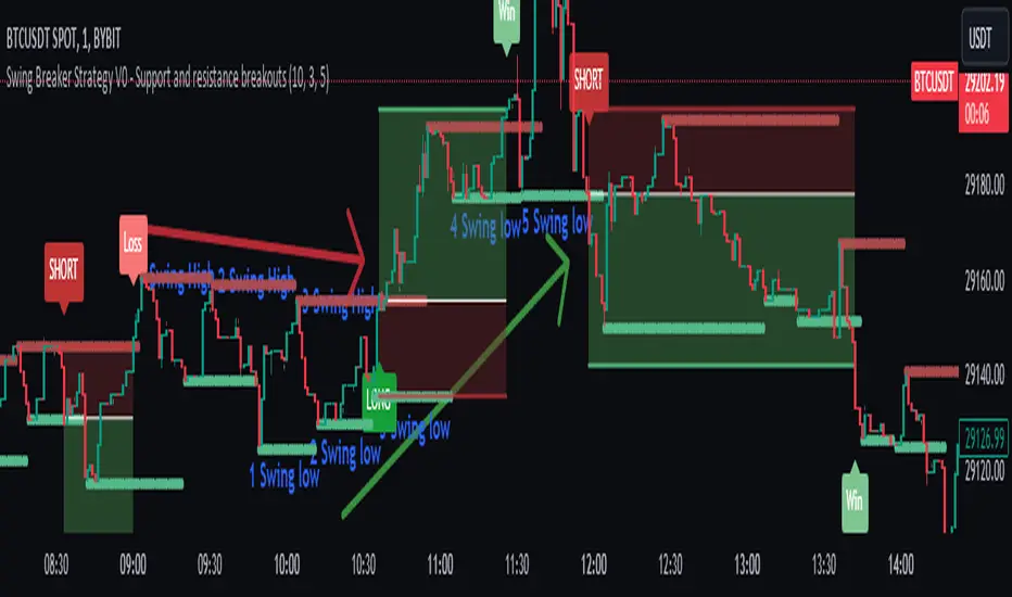
Blockunity Divinetrend (BDT)A formidable trend-following indicator, based on an ATR combined with a trailing stop mechanism. Divinetrend’s aim is to offer a simple and efficient alternative to Supertrend, another highly reputed indicator of the same type. It comes with a trading strategy that can be activated in its parameters. You can also change a number of design parameters.
Divinetrend is pretty straightforward in its approach. It calculates a base moving average taking into account the asset’s volatility, multiplies it with an ATR, then displays a line representing a trailing stop. When a red line is broken, the asset is considered to be moving back into an uptrend. Inversely, when a green line is broken, a bearish signal is sent. In the parameters, you can also activate a trend contestation period. If this parameter is activated, the price must have been trending for at least 5 days for the trend change to be validated.
Usage Advice
We recommend that you do not use this indicator with a time unit of less than 2 hours. Ideally in 4 hours or daily, or even 3 days. Otherwise, there’s nothing special about the use of this indicator. We still recommend that you use your logarithmic chart for a better visualization, but this is optional.
This indicator was designed in particular for the crypto market, but it also works on traditional market assets.
The Different Signals
Divinetrend gives buy and sell signals based on trailing stop line breaks and trend orientation. In particular, it can be used for trend identification and following. If the Contested Trend option is activated in the settings, the indicator will also display a contested period in blue. In this case, it is necessary to wait 5 days for the trend to be validated.
Integrated Strategy
In addition, a trading strategy is integrated into the Divinetrend indicator. This can be activated in the parameters. This is mainly there to see the results and the relevance of the indicator in the TradingView Strategy Tester. We do not recommend using it alone. As this strategy is used to study the indicator's performance, we use the following default parameters: An initial capital of 2,000 USDT with 100% of equity in order size. In other words, we'll bet the entire portfolio on each trade. To do this, we use a default stop loss of 10%, to avoid risking heavy losses. We also use a commission of 0.01% and a slippage of 3 ticks to reflect more reality.
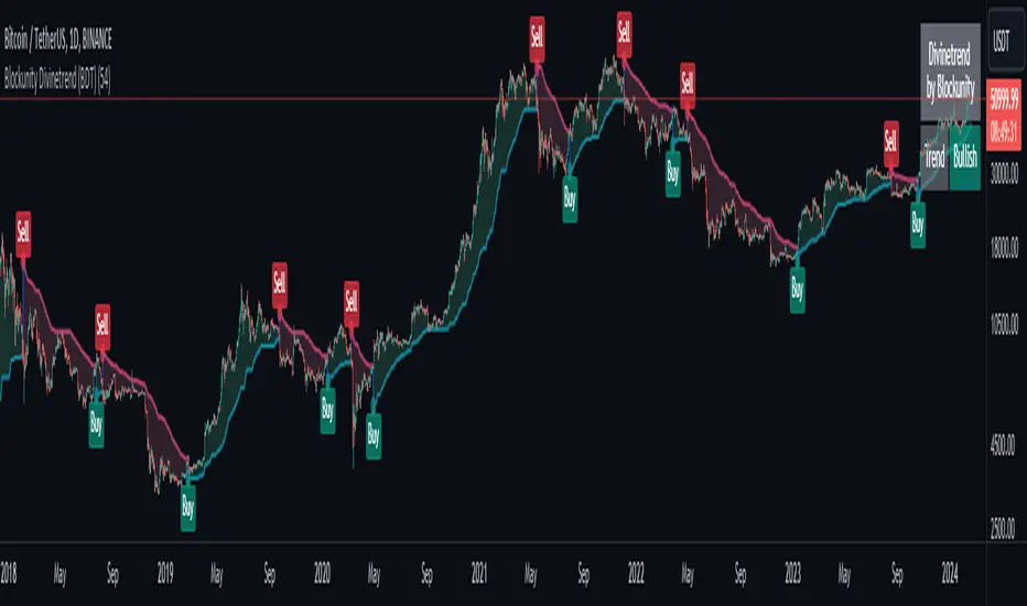
ELLIPSE: Bidirectional Swing Trading Strategy (Strategy Version)The eternal question that has occupied humanity since its early existence is what is the meaning of life and why am I here? On a daily basis this quest for meaning is distilled into a somewhat simpler question: What is the reason for getting up every morning?
For many of us, these thoughts arise even more as autumn arrives and it gets dark, bleak and cold outside. I guess it is easier to forget about the meaning of your life, while swimming on a sandy beach, enjoying a cocktail. Than you are living you life and you don’t need to rationalize it. Everything makes perfect sense!
In winter however, you need to get more “creative”. I, for example, would always try to change my perspective of things by doing something that makes my heart beat faster, like drinking a bottle of Heineken on a Friday evening or having endless conversations with my mates about stupid things, or kicking a ball against BALLONTHEROOF 7 on a Saturday morning. During the week, I would take out my frustrations on the fitness equipment at the local gym.
But what if all of this is canceled by CORONA? All that’s left is to work for the boss and run your 10km lap twice a week. The question is, what do you do now, with this huge amount of ”free” time than any old person would give anything for. When you are young time is never ending, when you are older it is never enough. Time has reached a different dimension in these days.
However, you can still do 2 things. You can slowly let the walls come to you and give up or you can actually do something useful with your time and find something that you are good at.
For us this choice was easy. After the success of our positioning trading strategy the MATRIX, at the time of the corona lockdown, we started making a swing trading strategy for the 4H timeframe, called ELLIPSE. We have included all feedback and any improvements we received about the positioning strategy and integrated it into the 4H script.
The main requirements of the script that we had set ourselves were:
Bidirectional
Low max drawdown
High profit factor
Works on all main crypto coins
By fully focusing ourselves on the script over the past few months, I can’t help but (unhumbly) say that we have not only succeeded in our mission, but that we have absolutely surpassed ourselves!
The only bright spot in this heavy corona time is, if a drug becomes available, there is extra money in the bank!
***The script is invite-only, message us to get script access***
-------------------------------------------------------------------------------------------------
User Guidelines:
The trading strategy was designed and optimized for trading cryptocurrencies only; furthermore it works best on established cryptocurrencies that have a clear historical trend such as:
BTCUSD
ETHUSD
LTCUSD
XRPUSD
ADAUSD
The trading strategy is based on swing trading methodology. The script must therefore be used on 4h candles only .
Use USD trading pairs only (e.g. use ETHUSD instead of the ETHBTC) since the individual trend is captured more effectively and therefore gives better results.
The trading strategy is bidirectional , both long and short entries are generated.
-------------------------------------------------------------------------------------------------
Indicators used in this strategy:
Ichimoku Cloud ; acts as the leading indicator.
Volume ; without strong volume , a market move is not valid.
MACD and Vortex ; both being used as confirmation indicators.
Choppiness index ; avoids trading in choppy markets.
Simple and Exponential Moving Averages ; prevents trading against the trend.
The trading strategy is easy to use, bidirectional, trend based and without repainting, meaning once a signal has been made it is permanent and that no future data is used in the decision making. It detects the trend and filters out market noise based on more than 10 technical indicators. ONLY when all indicators align with each other the algorithm prints a LONG or SHORT signal. The trading strategy provides high probability trading signals and minimizes risk! This script aims to capture the profit from short to medium trending moves and by doing so filters out non-substantial trends and avoids the associated risks with these trades.
-------------------------------------------------------------------------------------------------
Features:
NO Repaint once candle is closed.
Stop loss feature ; set your own stop loss to manage your risks.
Customizable Display for the Ichimoku cloud indicator display.
Bidirectional ; both long and short trading positions can be enabled.
Full backtest feature ; Easily generate your own backtest results for each asset (Strategy Version Script).
Alerts ; Get notified via email / pop-up / sms / app once a signal is given! (Alert Version Script).
-------------------------------------------------------------------------------------------------
Backtest results
Below are the back test results. Only well established cryptocurrencies are displayed with a clear historical trend:
Long and short trading positions,
Signal to signal trading (no multiple orders),
Initial Capital: 10 000 USD,
Order size: 10% of equity per trade,
commission fee 0.1%, period: start of chart,
Exchange-----Asset------Timeframe---Percent Profitable----Profit Factor---Total Trades----Max Drawdown----------Net Profit------
Bínance------BTCUSDT------4H-----------------54.4---------------5.32-----------------57----------------1.58%------------40.34%-(4034 USD)
Bínance------ETHUSD-------4H-----------------50.9---------------5.01---------------- 57----------------2.96%------------54.93%-(5493 USD)
Bínance------LTCUSD--------4H-----------------61.0---------------5.08-----------------59----------------2.09%------------57.06%-(5706 USD)
Bínance------XRPUSD-------4H-----------------43.13--------------3.52-----------------51----------------2.42%------------43.13%-(4313 USD)
Bínance------ADAUSD-------4H-----------------57.5---------------3.36-----------------47----------------3.46%------------40.82%-(4082 USD)
-------------------------------------------------------------------------------------------------
Reminder: Use this trading strategy at your own risk and trade responsibly. We are not responsible for any financial loss using this strategy.
***The script is invite-only, message us to get script access***

QuantNomad - SuperTrend - XBTUSD - 1mInteresting performance for Super Trend strategy for XBTUSD 1m chart.
Params: ST Mult: 2, ST Period 14.
Performance: 144% profit, 1988 trades, only 41% prof, 2.04% dd , 2.51 Sharpe.
On its own, it might be not a very good strategy, but the big amount of trades allows you to add more filters and improve it.
And remember:
Past performance does not guarantee future results.
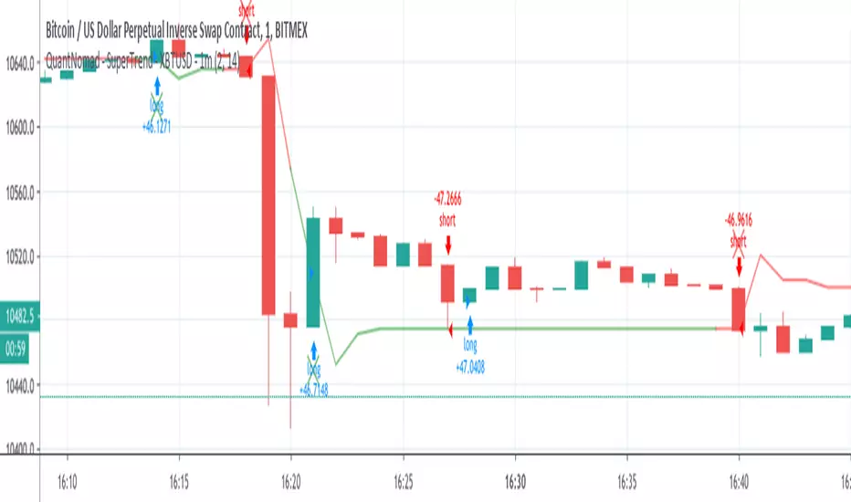
QuantNomad - SuperTrend - TSLA - 1mInteresting performance for Super Trend strategy for Tesla ( TSLA ) 1m chart.
Params: ST Mult: 3, ST Period 120.
Performance:61% profit, 637 trades, only 33% prof, 4.84% dd , 0.4 Sharpe.
On its own, it might be not a very good strategy, but the big amount of trades allows you to add more filters and improve it.
The strategy is not bad both with "when" params when strategy executed on open of next bar and with stop orders when strategy enters on exact Super Trend level.
You can comment/uncomment lines in the code and switch from one approach to another.
And remember:
Past performance does not guarantee future results.
