STD-Stepped Fast Cosine Transform Moving Average [Loxx]STD-Stepped Fast Cosine Transform Moving Average is an experimental moving average that uses Fast Cosine Transform to calculate a moving average. This indicator has standard deviation stepping in order to smooth the trend by weeding out low volatility movements.
What is the Discrete Cosine Transform?
A discrete cosine transform (DCT) expresses a finite sequence of data points in terms of a sum of cosine functions oscillating at different frequencies. The DCT, first proposed by Nasir Ahmed in 1972, is a widely used transformation technique in signal processing and data compression. It is used in most digital media, including digital images (such as JPEG and HEIF, where small high-frequency components can be discarded), digital video (such as MPEG and H.26x), digital audio (such as Dolby Digital, MP3 and AAC), digital television (such as SDTV, HDTV and VOD), digital radio (such as AAC+ and DAB+), and speech coding (such as AAC-LD, Siren and Opus). DCTs are also important to numerous other applications in science and engineering, such as digital signal processing, telecommunication devices, reducing network bandwidth usage, and spectral methods for the numerical solution of partial differential equations.
The use of cosine rather than sine functions is critical for compression, since it turns out (as described below) that fewer cosine functions are needed to approximate a typical signal, whereas for differential equations the cosines express a particular choice of boundary conditions. In particular, a DCT is a Fourier-related transform similar to the discrete Fourier transform (DFT), but using only real numbers. The DCTs are generally related to Fourier Series coefficients of a periodically and symmetrically extended sequence whereas DFTs are related to Fourier Series coefficients of only periodically extended sequences. DCTs are equivalent to DFTs of roughly twice the length, operating on real data with even symmetry (since the Fourier transform of a real and even function is real and even), whereas in some variants the input and/or output data are shifted by half a sample. There are eight standard DCT variants, of which four are common.
The most common variant of discrete cosine transform is the type-II DCT, which is often called simply "the DCT". This was the original DCT as first proposed by Ahmed. Its inverse, the type-III DCT, is correspondingly often called simply "the inverse DCT" or "the IDCT". Two related transforms are the discrete sine transform (DST), which is equivalent to a DFT of real and odd functions, and the modified discrete cosine transform (MDCT), which is based on a DCT of overlapping data. Multidimensional DCTs (MD DCTs) are developed to extend the concept of DCT to MD signals. There are several algorithms to compute MD DCT. A variety of fast algorithms have been developed to reduce the computational complexity of implementing DCT. One of these is the integer DCT (IntDCT), an integer approximation of the standard DCT, : ix, xiii, 1, 141–304 used in several ISO/IEC and ITU-T international standards.
Notable settings
windowper = period for calculation, restricted to powers of 2: "16", "32", "64", "128", "256", "512", "1024", "2048", this reason for this is FFT is an algorithm that computes DFT (Discrete Fourier Transform) in a fast way, generally in 𝑂(𝑁⋅log2(𝑁)) instead of 𝑂(𝑁2). To achieve this the input matrix has to be a power of 2 but many FFT algorithm can handle any size of input since the matrix can be zero-padded. For our purposes here, we stick to powers of 2 to keep this fast and neat. read more about this here: Cooley–Tukey FFT algorithm
smthper = smoothing count, this smoothing happens after the first FCT regular pass. this zeros out frequencies from the previously calculated values above SS count. the lower this number, the smoother the output, it works opposite from other smoothing periods
Included
Alerts
Signals
Loxx's Expanded Source Types
Additional reading
A Fast Computational Algorithm for the Discrete Cosine Transform by Chen et al.
Practical Fast 1-D DCT Algorithms With 11 Multiplications by Loeffler et al.
Cooley–Tukey FFT algorithm
Fourier

Real-Fast Fourier Transform of Price Oscillator [Loxx]Real-Fast Fourier Transform Oscillator is a simple Real-Fast Fourier Transform Oscillator. You have the option to turn on inverse filter as well as min/max filters to fine tune the oscillator. This oscillator is normalized by default. This indicator is to demonstrate how one can easily turn the RFFT algorithm into an oscillator..
What is the Discrete Fourier Transform?
In mathematics, the discrete Fourier transform (DFT) converts a finite sequence of equally-spaced samples of a function into a same-length sequence of equally-spaced samples of the discrete-time Fourier transform (DTFT), which is a complex-valued function of frequency. The interval at which the DTFT is sampled is the reciprocal of the duration of the input sequence. An inverse DFT is a Fourier series, using the DTFT samples as coefficients of complex sinusoids at the corresponding DTFT frequencies. It has the same sample-values as the original input sequence. The DFT is therefore said to be a frequency domain representation of the original input sequence. If the original sequence spans all the non-zero values of a function, its DTFT is continuous (and periodic), and the DFT provides discrete samples of one cycle. If the original sequence is one cycle of a periodic function, the DFT provides all the non-zero values of one DTFT cycle.
What is the Complex Fast Fourier Transform?
The complex Fast Fourier Transform algorithm transforms N real or complex numbers into another N complex numbers. The complex FFT transforms a real or complex signal x in the time domain into a complex two-sided spectrum X in the frequency domain. You must remember that zero frequency corresponds to n = 0, positive frequencies 0 < f < f_c correspond to values 1 ≤ n ≤ N/2 −1, while negative frequencies −fc < f < 0 correspond to N/2 +1 ≤ n ≤ N −1. The value n = N/2 corresponds to both f = f_c and f = −f_c. f_c is the critical or Nyquist frequency with f_c = 1/(2*T) or half the sampling frequency. The first harmonic X corresponds to the frequency 1/(N*T).
The complex FFT requires the list of values (resolution, or N) to be a power 2. If the input size if not a power of 2, then the input data will be padded with zeros to fit the size of the closest power of 2 upward.
What is Real-Fast Fourier Transform?
Has conditions similar to the complex Fast Fourier Transform value, except that the input data must be purely real. If the time series data has the basic type complex64, only the real parts of the complex numbers are used for the calculation. The imaginary parts are silently discarded.
Included
Moving window from Last Bar setting. You can lock the oscillator in place on the current bar by adding 1 every time a new bar appears in the Last Bar Setting

Real-Fast Fourier Transform of Price w/ Linear Regression [Loxx]Real-Fast Fourier Transform of Price w/ Linear Regression is a indicator that implements a Real-Fast Fourier Transform on Price and modifies the output by a measure of Linear Regression. The solid line is the Linear Regression Trend of the windowed data, The green/red line is the Real FFT of price.
What is the Discrete Fourier Transform?
In mathematics, the discrete Fourier transform (DFT) converts a finite sequence of equally-spaced samples of a function into a same-length sequence of equally-spaced samples of the discrete-time Fourier transform (DTFT), which is a complex-valued function of frequency. The interval at which the DTFT is sampled is the reciprocal of the duration of the input sequence. An inverse DFT is a Fourier series, using the DTFT samples as coefficients of complex sinusoids at the corresponding DTFT frequencies. It has the same sample-values as the original input sequence. The DFT is therefore said to be a frequency domain representation of the original input sequence. If the original sequence spans all the non-zero values of a function, its DTFT is continuous (and periodic), and the DFT provides discrete samples of one cycle. If the original sequence is one cycle of a periodic function, the DFT provides all the non-zero values of one DTFT cycle.
What is the Complex Fast Fourier Transform?
The complex Fast Fourier Transform algorithm transforms N real or complex numbers into another N complex numbers. The complex FFT transforms a real or complex signal x in the time domain into a complex two-sided spectrum X in the frequency domain. You must remember that zero frequency corresponds to n = 0, positive frequencies 0 < f < f_c correspond to values 1 ≤ n ≤ N/2 −1, while negative frequencies −fc < f < 0 correspond to N/2 +1 ≤ n ≤ N −1. The value n = N/2 corresponds to both f = f_c and f = −f_c. f_c is the critical or Nyquist frequency with f_c = 1/(2*T) or half the sampling frequency. The first harmonic X corresponds to the frequency 1/(N*T).
The complex FFT requires the list of values (resolution, or N) to be a power 2. If the input size if not a power of 2, then the input data will be padded with zeros to fit the size of the closest power of 2 upward.
What is Real-Fast Fourier Transform?
Has conditions similar to the complex Fast Fourier Transform value, except that the input data must be purely real. If the time series data has the basic type complex64, only the real parts of the complex numbers are used for the calculation. The imaginary parts are silently discarded.
Inputs:
src = source price
uselreg = whether you wish to modify output with linear regression calculation
Windowin = windowing period, restricted to powers of 2: "4", "8", "16", "32", "64", "128", "256", "512", "1024", "2048"
Treshold = to modified power output to fine tune signal
dtrendper = adjust regression calculation
barsback = move window backward from bar 0
mutebars = mute bar coloring for the range
Further reading:
Real-valued Fast Fourier Transform Algorithms IEEE Transactions on Acoustics, Speech, and Signal Processing, June 1987
Related indicators utilizing Fourier Transform
Fourier Extrapolator of Variety RSI w/ Bollinger Bands
Fourier Extrapolation of Variety Moving Averages
Fourier Extrapolator of Price w/ Projection Forecast

Variety RSI of Fast Discrete Cosine Transform [Loxx]Variety RSI of Fast Discrete Cosine Transform is an RSI indicator with 7 types of RSI that is calculated on the Fast Discrete Cosine Transform of source. The source inputs are 33 different source types from Loxx's Expanded Source Types.
What is Discrete Cosine Transform?
A discrete cosine transform (DCT) expresses a finite sequence of data points in terms of a sum of cosine functions oscillating at different frequencies. The DCT, first proposed by Nasir Ahmed in 1972, is a widely used transformation technique in signal processing and data compression. It is used in most digital media, including digital images (such as JPEG and HEIF, where small high-frequency components can be discarded), digital video (such as MPEG and H.26x), digital audio (such as Dolby Digital, MP3 and AAC), digital television (such as SDTV, HDTV and VOD), digital radio (such as AAC+ and DAB+), and speech coding (such as AAC-LD, Siren and Opus). DCTs are also important to numerous other applications in science and engineering, such as digital signal processing, telecommunication devices, reducing network bandwidth usage, and spectral methods for the numerical solution of partial differential equations.
Fast Discrete Cosine Transform
The algorithm performs a fast cosine transform of the real function defined by nn samples on the real axis.
Depending on the passed parameters, it can be executed both direct and inverse conversion.
Input parameters:
tnn - Number of function values minus one. Should be 1024 degree of two. The algorithm does not check correct value passed.
a - array of Real 1025 Function values.
InverseFCT - the direction of the transformation. True if reverse, False if direct.
Output parameters: a - the result of the transformation. For more details, see description on the site. www.alglib.net
Included:
7 types of RSI
33 source inputs from Loxx's Expanded Source Types
2 types of signals
Alerts
Fourier Extrapolation of Variety Moving Averages [Loxx]Fourier Extrapolation of Variety Moving Averages is a Fourier Extrapolation (forecasting) indicator that has for inputs 38 different types of moving averages along with 33 different types of sources for those moving averages. This is a forecasting indicator of the selected moving average of the selected price of the underlying ticker. This indicator will repaint, so past signals are only as valid as the current bar. This indicator allows for up to 1500 bars between past bars and future projection bars. If the indicator won't load on your chart. check the error message for details on how to fix that, but you must ensure that past bars + futures bars is equal to or less than 1500.
Fourier Extrapolation using the Quinn-Fernandes algorithm is one of several (5-10) methods of signals forecasting that I'l be demonstrating in Pine Script.
What is Fourier Extrapolation?
This indicator uses a multi-harmonic (or multi-tone) trigonometric model of a price series xi, i=1..n, is given by:
xi = m + Sum( a*Cos(w*i) + b*Sin(w*i), h=1..H )
Where:
xi - past price at i-th bar, total n past prices;
m - bias;
a and b - scaling coefficients of harmonics;
w - frequency of a harmonic ;
h - harmonic number;
H - total number of fitted harmonics.
Fitting this model means finding m, a, b, and w that make the modeled values to be close to real values. Finding the harmonic frequencies w is the most difficult part of fitting a trigonometric model. In the case of a Fourier series, these frequencies are set at 2*pi*h/n. But, the Fourier series extrapolation means simply repeating the n past prices into the future.
This indicator uses the Quinn-Fernandes algorithm to find the harmonic frequencies. It fits harmonics of the trigonometric series one by one until the specified total number of harmonics H is reached. After fitting a new harmonic , the coded algorithm computes the residue between the updated model and the real values and fits a new harmonic to the residue.
see here: A Fast Efficient Technique for the Estimation of Frequency , B. G. Quinn and J. M. Fernandes, Biometrika, Vol. 78, No. 3 (Sep., 1991), pp . 489-497 (9 pages) Published By: Oxford University Press
The indicator has the following input parameters:
src - input source
npast - number of past bars, to which trigonometric series is fitted;
Nfut - number of predicted future bars;
nharm - total number of harmonics in model;
frqtol - tolerance of frequency calculations.
Included:
Loxx's Expanded Source Types
Loxx's Moving Averages
Other indicators using this same method
Fourier Extrapolator of Variety RSI w/ Bollinger Bands
Fourier Extrapolator of Price w/ Projection Forecast
Fourier Extrapolator of Price
Loxx's Moving Averages: Detailed explanation of moving averages inside this indicator
Loxx's Expanded Source Types: Detailed explanation of source types used in this indicator
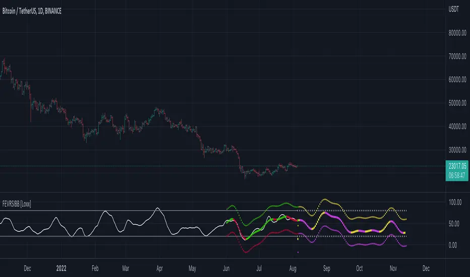
Fourier Extrapolator of Variety RSI w/ Bollinger Bands [Loxx]Fourier Extrapolator of Variety RSI w/ Bollinger Bands is an RSI indicator that shows the original RSI, the Fourier Extrapolation of RSI in the past, and then the projection of the Fourier Extrapolated RSI for the future. This indicator has 8 different types of RSI including a new type of RSI called T3 RSI. The purpose of this indicator is to demonstrate the Fourier Extrapolation method used to model past data and to predict future price movements. This indicator will repaint. If you wish to use this for trading, then make sure to take a screenshot of the indicator when you enter the trade to save your analysis. This is the first of a series of forecasting indicators that can be used in trading. Due to how this indicator draws on the screen, you must choose values of npast and nfut that are equal to or less than 200. this is due to restrictions by TradingView and Pine Script in only allowing 500 lines on the screen at a time. Enjoy!
What is Fourier Extrapolation?
This indicator uses a multi-harmonic (or multi-tone) trigonometric model of a price series xi, i=1..n, is given by:
xi = m + Sum( a*Cos(w*i) + b*Sin(w*i), h=1..H )
Where:
xi - past price at i-th bar, total n past prices;
m - bias;
a and b - scaling coefficients of harmonics;
w - frequency of a harmonic ;
h - harmonic number;
H - total number of fitted harmonics.
Fitting this model means finding m, a, b, and w that make the modeled values to be close to real values. Finding the harmonic frequencies w is the most difficult part of fitting a trigonometric model. In the case of a Fourier series, these frequencies are set at 2*pi*h/n. But, the Fourier series extrapolation means simply repeating the n past prices into the future.
This indicator uses the Quinn-Fernandes algorithm to find the harmonic frequencies. It fits harmonics of the trigonometric series one by one until the specified total number of harmonics H is reached. After fitting a new harmonic , the coded algorithm computes the residue between the updated model and the real values and fits a new harmonic to the residue.
see here: A Fast Efficient Technique for the Estimation of Frequency , B. G. Quinn and J. M. Fernandes, Biometrika, Vol. 78, No. 3 (Sep., 1991), pp . 489-497 (9 pages) Published By: Oxford University Press
The indicator has the following input parameters:
src - input source
npast - number of past bars, to which trigonometric series is fitted;
Nfut - number of predicted future bars;
nharm - total number of harmonics in model;
frqtol - tolerance of frequency calculations.
Included:
Loxx's Expanded Source Types
Loxx's Variety RSI
Other indicators using this same method
Fourier Extrapolator of Price w/ Projection Forecast
Fourier Extrapolator of Price
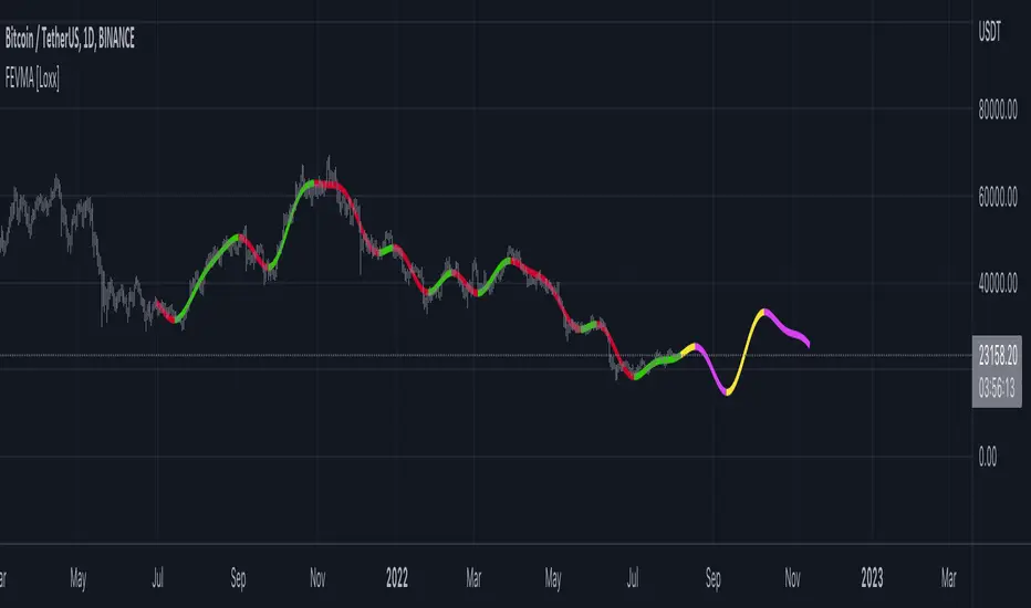
Fourier Extrapolator of Price w/ Projection Forecast [Loxx]Due to popular demand, I'm pusblishing Fourier Extrapolator of Price w/ Projection Forecast.. As stated in it's twin indicator, this one is also multi-harmonic (or multi-tone) trigonometric model of a price series xi, i=1..n, is given by:
xi = m + Sum( a*Cos(w*i) + b*Sin(w*i), h=1..H )
Where:
xi - past price at i-th bar, total n past prices;
m - bias;
a and b - scaling coefficients of harmonics;
w - frequency of a harmonic ;
h - harmonic number;
H - total number of fitted harmonics.
Fitting this model means finding m, a, b, and w that make the modeled values to be close to real values. Finding the harmonic frequencies w is the most difficult part of fitting a trigonometric model. In the case of a Fourier series, these frequencies are set at 2*pi*h/n. But, the Fourier series extrapolation means simply repeating the n past prices into the future.
This indicator uses the Quinn-Fernandes algorithm to find the harmonic frequencies. It fits harmonics of the trigonometric series one by one until the specified total number of harmonics H is reached. After fitting a new harmonic , the coded algorithm computes the residue between the updated model and the real values and fits a new harmonic to the residue.
see here: A Fast Efficient Technique for the Estimation of Frequency , B. G. Quinn and J. M. Fernandes, Biometrika, Vol. 78, No. 3 (Sep., 1991), pp . 489-497 (9 pages) Published By: Oxford University Press
The indicator has the following input parameters:
src - input source
npast - number of past bars, to which trigonometric series is fitted;
Nfut - number of predicted future bars;
nharm - total number of harmonics in model;
frqtol - tolerance of frequency calculations.
The indicator plots two curves: the green/red curve indicates modeled past values and the yellow/fuchsia curve indicates the modeled future values.
The purpose of this indicator is to showcase the Fourier Extrapolator method to be used in future indicators.

Fourier Extrapolator of Price [Loxx]Fourier Extrapolator of Price is a multi-harmonic (or multi-tone) trigonometric model of a price series xi, i=1..n, is given by:
xi = m + Sum( a *Cos(w *i) + b *Sin(w *i), h=1..H )
Where:
xi - past price at i-th bar, total n past prices;
m - bias;
a and b - scaling coefficients of harmonics;
w - frequency of a harmonic;
h - harmonic number;
H - total number of fitted harmonics.
Fitting this model means finding m, a , b , and w that make the modeled values to be close to real values. Finding the harmonic frequencies w is the most difficult part of fitting a trigonometric model. In the case of a Fourier series, these frequencies are set at 2*pi*h/n. But, the Fourier series extrapolation means simply repeating the n past prices into the future.
This indicator uses the Quinn-Fernandes algorithm to find the harmonic frequencies. It fits harmonics of the trigonometric series one by one until the specified total number of harmonics H is reached. After fitting a new harmonic, the coded algorithm computes the residue between the updated model and the real values and fits a new harmonic to the residue.
see here: A Fast Efficient Technique for the Estimation of Frequency , B. G. Quinn and J. M. Fernandes, Biometrika, Vol. 78, No. 3 (Sep., 1991), pp. 489-497 (9 pages) Published By: Oxford University Press
The indicator has the following input parameters:
src - input source
npast - number of past bars, to which trigonometric series is fitted;
nharm - total number of harmonics in model;
frqtol - tolerance of frequency calculations.
The indicator plots the modeled past values
The purpose of this indicator is to showcase the Fourier Extrapolator method to be used in future indicators. While this method can also prediction future price movements, for our purpose here we will avoid doing.

OPAL - Sense→ Hi everyone, very proud to publish my unique leading oscillator ! ←
Sense is a "leading indicator" : it shows what can happen in the future, meanwhile a lagging indicator like MAs shows past sentiment.
Sense diverging with Price ? Care at the reversal !
It can be a great tool to upgrade your timings, after a divergence for example, to snipe reversals or to find Trend entries.
This tool is used for sniping in our levels trading setup (in our trading community)
Sense is made of everything you know about common indicators :
RSI/STOCH/STOCHRSI/MFI/RVSI/PZO/VZO/MOMENTUM/VOLUMES/UO
>>> Basically shows situations where almost all the known indicators reach interesting points in Overbought and Oversold zones
Signals provided :
*Visible and Hidden Minor OB/OS Crosses (Small Arrows)
*Visible and Hidden Major OB/OS Crosses (Bigger Arrows)
*Visible and Hidden Major and Minor Confluence in OB/OS Zones (Rockets/Blood)
*Background Smart Coloring when price reaches OB/OS Zones :
- blue/purple = entering OB/OS Zones
- green/red = extrem multiple OB/OS situation
*Coloration of Middle Line based on std Price Deviation
*Smart Divergences spotting : applied level filter to get divergences that reached OB/OS Zones at least once.
Divergences are scanned twice for confirmation<
*Full alerting system on :
- Full signals = blood and rockets
- Half signals = bigger arrows
- Minor signals = small arrows
- Dual Divergences = on both oscillators (slow & fast)
1) What is the curve i see on Sense ? => It is my homemade oscillator, described above
2) What are thoses Zones around the curve ? => Overbought/Oversold Zones
3) What are those dots on the curve ? => When the oscillator crosses its Triggerline
4) What are those little arrows ? => Printing minor Overbought/Oversold situations
5) What are those bigger arrows ? => Printing major Overbought/Oversold situations
6) What are those Blood dots/ Rockets ? => Printing Confluence situations in Overbought/Oversold Zones
7) Why is background coloring ? => I applied smart coloration based on oscillators location (see above coloration meaning)
8) What are those lines between curve spikes ? => Situations when Price and oscillator are doing different moves, basically divergences, meaning a correction can happen sooner or later
Should be strong on almost every timeframe !
Always backtest, watch, then use or not in your trading strategy.
If you like my work, leave a like :)
Hoping you success !

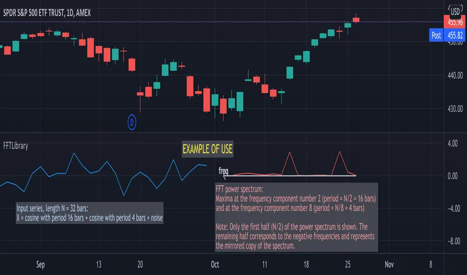
FFTLibraryLibrary "FFTLibrary" contains a function for performing Fast Fourier Transform (FFT) along with a few helper functions. In general, FFT is defined for complex inputs and outputs. The real and imaginary parts of formally complex data are treated as separate arrays (denoted as x and y). For real-valued data, the array of imaginary parts should be filled with zeros.
FFT function
fft(x, y, dir) : Computes the one-dimensional discrete Fourier transform using an in-place complex-to-complex FFT algorithm . Note: The transform also produces a mirror copy of the frequency components, which correspond to the signal's negative frequencies.
Parameters:
x : float array, real part of the data, array size must be a power of 2
y : float array, imaginary part of the data, array size must be the same as x ; for real-valued input, y must be an array of zeros
dir : string, options = , defines the direction of the transform: forward" (time-to-frequency) or inverse (frequency-to-time)
Returns: x, y : tuple (float array, float array), real and imaginary parts of the transformed data (original x and y are changed on output)
Helper functions
fftPower(x, y) : Helper function that computes the power of each frequency component (in other words, Fourier amplitudes squared).
Parameters:
x : float array, real part of the Fourier amplitudes
y : float array, imaginary part of the Fourier amplitudes
Returns: power : float array of the same length as x and y , Fourier amplitudes squared
fftFreq(N) : Helper function that returns the FFT sample frequencies defined in cycles per timeframe unit. For example, if the timeframe is 5m, the frequencies are in cycles/(5 minutes).
Parameters:
N : int, window length (number of points in the transformed dataset)
Returns: freq : float array of N, contains the sample frequencies (with zero at the start).
Function Sawtooth WaveThis is an indicator to draw a sawtooth wave on the chart.
It can be a useful perspective, as decaying markets tend to oscillate in reverse sawtooth waves, and bullish markets can oscillate in conventional sawtooth waves. With the right inputs, it can be an early warning signal for potential movements.
Something I've noted is that large waves cause a ripple effect and sets the frequency for the market until a change occurs. Sawtooth waves may help in capturing ripple waves.
Useful inputs are:
- Average True Range as wave height (amplitude)
- Periodicity of market as wave duration (frequency)
(Inputs will change the wave from conventional to reverse)
I hope that it is helpful.
GLHF
- DPT

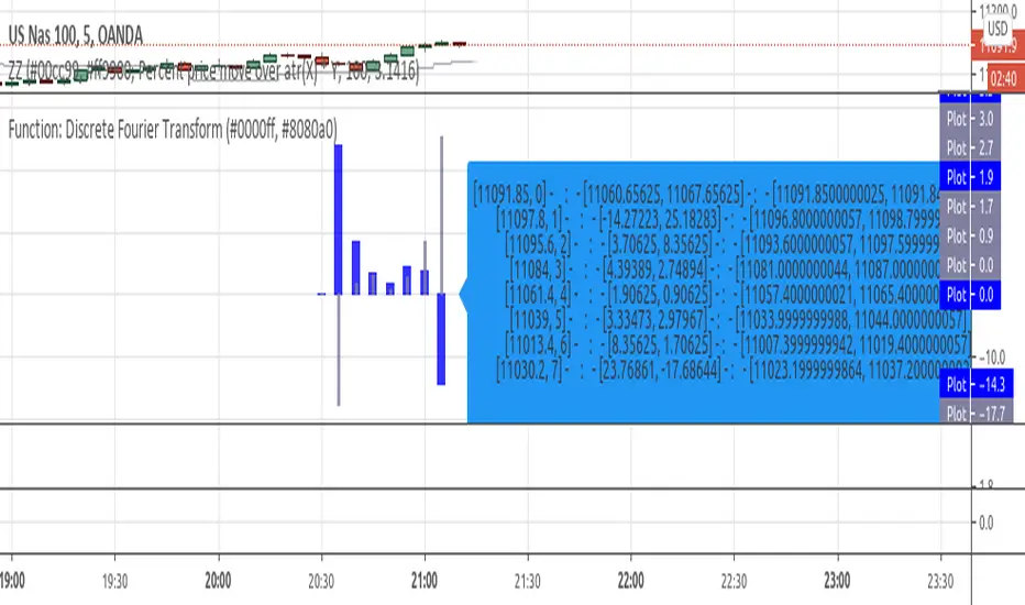
Function: Discrete Fourier TransformExperimental:
function for inverse and discrete fourier transform in one, if you notice errors please let me know! use at your own risk...
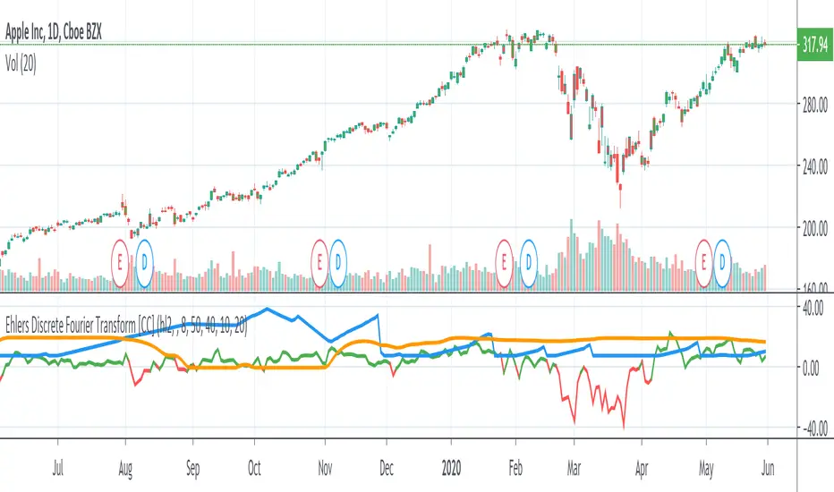
Ehlers Discrete Fourier TransformThe Discrete Fourier Transform Indicator was written by John Ehlers and more details can be found at www.mesasoftware.com
I have color coded everything as follows: blue line is the dominant cycle, orange line is the power converted to decibels, and I have marked the other line as red if you should sell or green if you should buy
Let me know if you would like to see me write any other scripts!
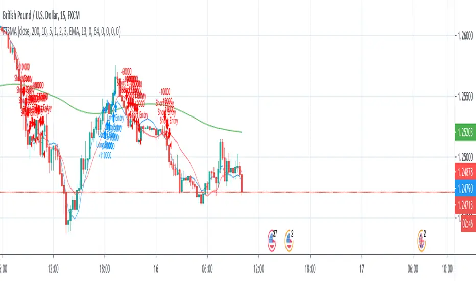
FTSMA - Trend is your frendThis my new solid strategy: if you belive that "TREND IS YOUR FRIEND" this is for you!
I have tested with many pairs and at many timeframes and have profit with just minor changes in settings.
I suggest to use it for intraday trading .
VERY IMPORTANT NOTE: this is a trend following strategy, so the target is to stay in the trade as much as possible. If your trading style is more focused on scalping and/or pullbaks, this strategy is not for you.
This strategy uses moving averages applied to Fourier waves for forecasting trend direction.
How strategy works:
- Buy when fast MA is above mid MA and price is above slow MA, which acts as a trend indicator.
- Sell when fast MA is below mid MA and price is below slow MA, which acts as a trend indicator.
Strategy uses a lot of pyramiding orders because when you are in a flat market phase it will close 1 or 2 orders with a loss, but when a big trend starts, it will have profit in a lot of orders.
So, if you analize carefully the strategy results, you will note that "Percent Profitable" is very low (30% in this case) because strategy opened a lot of orders also in flat markets with small losses, BUT "Avg # bars in winning trades" is very high and overall Profit is very high: when a big trend starts, orders are kept open for long time generating big profits.
Thanks to all pinescripters mentioned in the code for their snippets.
I have also a study with alerts. Next improvement (only to whom is interested to this script and follows me): study with alerts on multiple tickers all at one. Leave a comment if you want to have access to study.
HOW TO USE STRATEGY AND STUDY TOGHETER:
1- Add to chart the strategy first, so your workspace will be as clean as possible.
2- Open the Strategy Tester tab at footer of the page.
3- Modify settings to get best results (Profit, Profit Factor, Drawdown).
4- Add study with alerts to your chart with same setting of strategy.
I WILL PROVIDE A DETAILED QUICK INSTALLATION GUIDE WITH THE STUDY!
Please use comment section for any feedback or contact me if you need support.
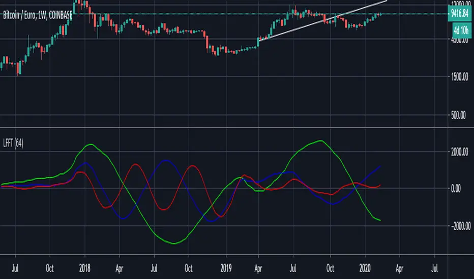
Low Frequency Fourier TransformThis Study uses the Real Discrete Fourier Transform algorithm to generate 3 sinusoids possibly indicative of future price.
I got information about this RDFT algorithm from "The Scientist and Engineer's Guide to Digital Signal Processing" By Steven W. Smith, Ph.D.
It has not been tested thoroughly yet, but it seems that that the RDFT isn't suited for predicting prices as the Frequency Domain Representation shows that the signal is similar to white noise, showing no significant peaks, indicative of very low periodicity of price movements.
Fourier series Model Of The Market█ OVERVIEW
The Fourier Series Model of the Market (FSMM) decomposes price action into harmonic components using bandpass filtering, then reconstructs a composite wave weighted by rolling energy ratios. This approach isolates cyclical market behavior at multiple frequencies, emphasizing dominant cycles for cleaner signal generation. The energy-adaptive weighting is the key differentiator from simple harmonic summation: cycles that dominate current price action contribute more to the output.
Based on Fourier analysis principles applied to financial markets, the indicator extracts harmonics (fundamental, 2nd, 3rd, etc.) using second-order IIR bandpass filters, then weights each harmonic's contribution by its relative energy compared to adjacent harmonics. This energy-adaptive weighting naturally emphasizes the cycles that are most prominent in current market conditions.
█ CONCEPTS
Fourier Decomposition
Fourier analysis represents any periodic signal as a sum of sine waves at different frequencies. In market analysis, price action can be decomposed into a fundamental cycle (the base period) plus harmonics at integer multiples of that frequency (period/2, period/3, etc.). Each harmonic captures oscillations at a specific frequency band, and their sum reconstructs the original cyclical behavior.
Bandpass Filtering
Each harmonic is extracted using a second-order IIR (Infinite Impulse Response) bandpass filter tuned to that harmonic's frequency. The filter isolates price activity within a narrow frequency range while rejecting both higher-frequency noise and lower-frequency trend drift. Before filtering, the source is debiased via 2-bar momentum to remove DC offset, ensuring each bandpass operates around true zero.
Energy-Weighted Reconstruction
Rather than simply summing all harmonics equally, FSMM weights each harmonic by its rolling energy relative to the previous harmonic. The energy score combines the current harmonic value with its rate of change, so it reflects both amplitude and momentum. Higher harmonics that hold comparatively more energy therefore contribute more to the composite wave, while weaker harmonics fade out. This adaptive weighting allows the model to respond to changing market cyclicality.
Quadrature Component (Rate of Change)
The rate of change output represents the 90°-phase-shifted (quadrature) component of the wave. When the wave is at zero and rising, the rate of change is at maximum positive. This provides complementary information about cycle phase and can be used for timing entries relative to cycle position.
█ INTERPRETATION
Wave Output
The composite wave oscillates around zero, representing the sum of all extracted harmonic components weighted by energy:
• Above zero : Net bullish cyclical momentum across harmonics
• Below zero : Net bearish cyclical momentum across harmonics
• Zero crossings : Cycle phase transitions - potential reversal points
• Wave amplitude : Strength of cyclical behavior; larger swings indicate cleaner cycles
Rate of Change
The quadrature component (90° phase-shifted) provides cycle phase information:
• Maximum rate of change : Wave is near zero and accelerating - early cycle phase
• Zero rate of change : Wave is at peak or trough - cycle extremes
• Rate/Wave divergence : When wave makes new highs/lows but rate of change does not confirm (lower momentum), suggests cycle exhaustion or impending phase shift
Combined Analysis
• Wave crossing above zero with positive rate of change: Strong bullish cycle initiation
• Wave crossing below zero with negative rate of change: Strong bearish cycle initiation
• Wave at extreme with rate of change reversing: Potential cycle peak/trough
Threshold Bands
When enabled, threshold bands define statistically significant wave deviations:
• Breach above +threshold : Unusually strong bullish cyclical behavior
• Breach below -threshold : Unusually strong bearish cyclical behavior
• Return inside thresholds : Normalizing behavior, potential mean reversion ahead
Alert Conditions
Four built-in alerts trigger on bar close (no repainting):
• Above +Threshold : Strong bullish cycle behavior
• Below -Threshold : Strong bearish cycle behavior
• Above Zero : Bullish cycle phase shift
• Below Zero : Bearish cycle phase shift
█ SETTINGS & PARAMETER TUNING
Fourier Series Model
• Source : Price series to decompose into harmonic components.
• Period (6-100): Base period for the fundamental harmonic. Higher harmonics divide this period (harmonic 2 = period/2, harmonic 3 = period/3). Match to the dominant market cycle for best results. Default 20.
• Bandwidth (0.05-0.5): Bandpass filter selectivity. Lower values create narrower passbands that isolate harmonics more precisely but may miss slightly off-frequency cycles. Higher values capture broader ranges but reduce harmonic separation. Default 0.1 balances precision and robustness.
• Harmonics (1-20): Number of harmonic components to extract. More harmonics capture finer cyclical detail but increase computation. For most applications, 3-5 harmonics suffice. The fundamental alone (1 harmonic) functions as a simple bandpass filter.
Display Settings
• Wave Outputs : Toggle visibility and color of the composite Fourier wave.
• Rate of Change : Toggle visibility and color of the quadrature component (90° phase-shifted wave).
• Zero Line : Reference line for oscillator neutrality.
Diagnostics - Dynamic Thresholds
Optional significance bands that identify when wave readings indicate strong cyclical behavior:
• Dynamic Threshold : Toggle threshold bands and set colors.
• Threshold Mode : Select calculation method:
- MAD (Median Absolute Deviation) : Robust, outlier-resistant measure using k * MAD where MAD ≈ 0.6745 * stdev.
- Standard Deviation : Volatility-sensitive, calculated as k * stdev of wave over the lookback period.
- Percentile Rank : Fixed probability bands using percentile of |wave| (90% means only 10% of values exceed threshold).
• Period (2-200): Lookback for threshold calculations. Default 50.
• Multiplier (k) : Scaling for MAD/Standard Deviation modes. Default 1.5.
• Percentile (%) (0-100): For Percentile Rank mode only. Default 90%.
Parameter Interactions
• Shorter periods respond faster to cycle changes but may capture noise.
• Lower bandwidth + more harmonics = more precise decomposition but requires accurate period setting.
• Higher bandwidth is more forgiving of period mismatches.
• For strongly trending markets, restrict harmonics to 1-2 so the model tracks the dominant cycle with fewer higher-frequency components.
• For ranging/oscillating markets, more harmonics (4-6) capture complex cycles.
█ LIMITATIONS
Inherent Characteristics
• Period dependency : Effectiveness depends on correctly matching the Period parameter to actual market cycles. Use cycle measurement tools (autocorrelation, FFT, dominant cycle indicators) to identify appropriate periods.
• Stationarity assumption : The indicator assumes cycle frequencies remain relatively stable within the lookback window. Rapidly shifting dominant cycles (regime transitions) may produce inconsistent results until the buffer adapts.
• Filter lag : Despite bandpass design, some lag remains inherent to causal filtering. Higher harmonics have less lag but more noise sensitivity.
• Energy weighting artifacts : During regime changes when harmonic energy ratios shift rapidly, weighting may produce transient anomalies.
Market Conditions to Avoid
• Strong trending markets : Pure trends with no cyclicality produce weak, meandering signals. The indicator assumes cyclical market behavior.
• News events/gaps : Large discontinuities disrupt filter continuity. Requires 1-2 full periods to stabilize.
• Period mismatch : If the Period parameter doesn't match actual market cycles, harmonic extraction produces noise rather than signal.
Parameter Selection Pitfalls
• Too many harmonics : Beyond 5-6 harmonics, additional components often capture noise rather than meaningful cycles.
• Bandwidth too narrow : Very low bandwidth (< 0.05) requires extremely precise period matching; slight mismatches cause signal loss.
• Over-optimization : Perfect historical parameter fits typically fail forward. Use robust defaults across multiple instruments.
█ NOTES
Credits
This indicator applies Fourier analysis principles to financial market data, building on the extensive work of Dr. John F. Ehlers in applying digital signal processing to trading. The bandpass filter implementation and harmonic decomposition approach draw from DSP fundamentals as presented in Ehlers' publications.
For those interested in the underlying mathematics and DSP concepts:
• Ehlers, J.F. (2001). Rocket Science for Traders: Digital Signal Processing Applications . John Wiley & Sons.
• Ehlers, J.F. (2013). Cycle Analytics for Traders . John Wiley & Sons.
• Various TASC articles by John Ehlers on bandpass filters, cycle analysis, and harmonic decomposition.
by ♚@e2e4

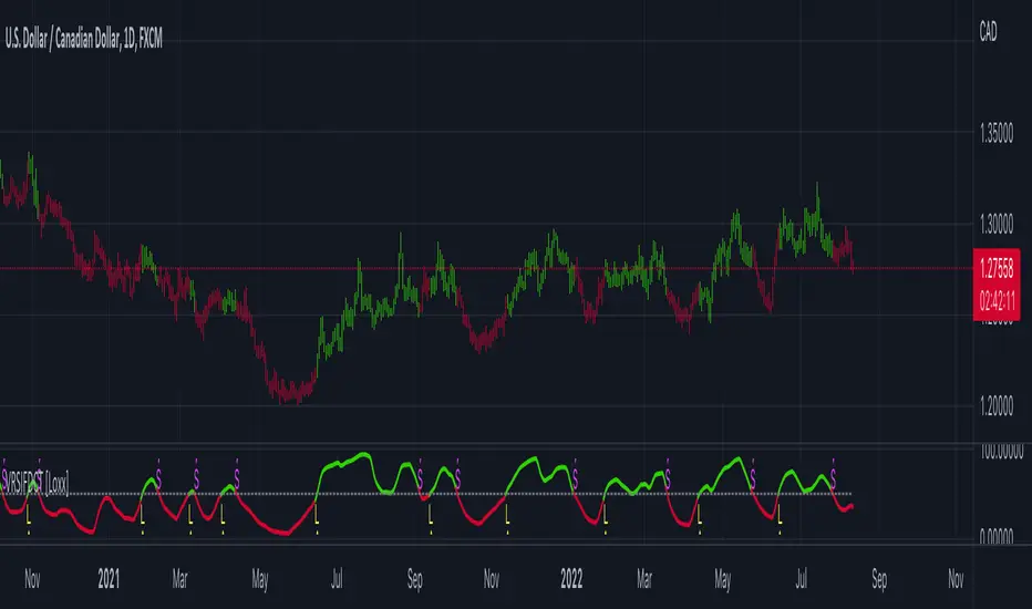
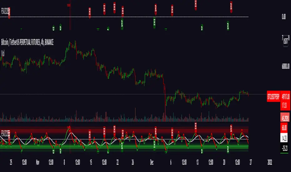
Regularized Volume Zone Oscillator FSVZORegularized VZO
Vanilla in link below
White noise and 1 confirm auto divs included
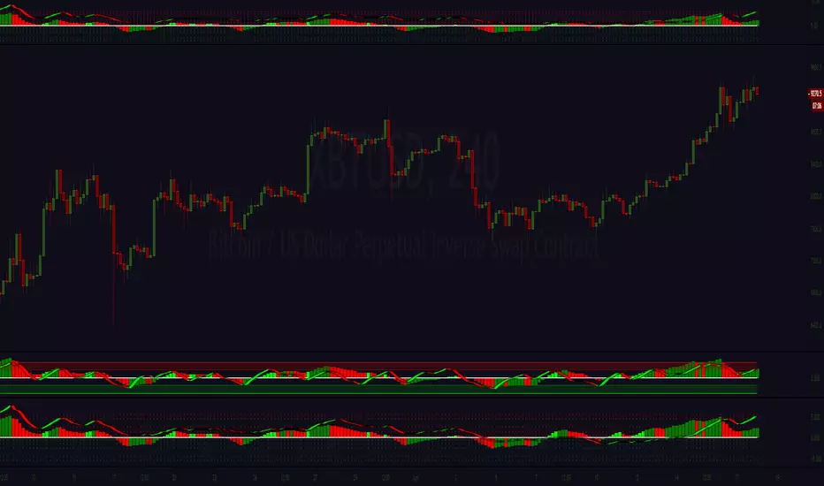
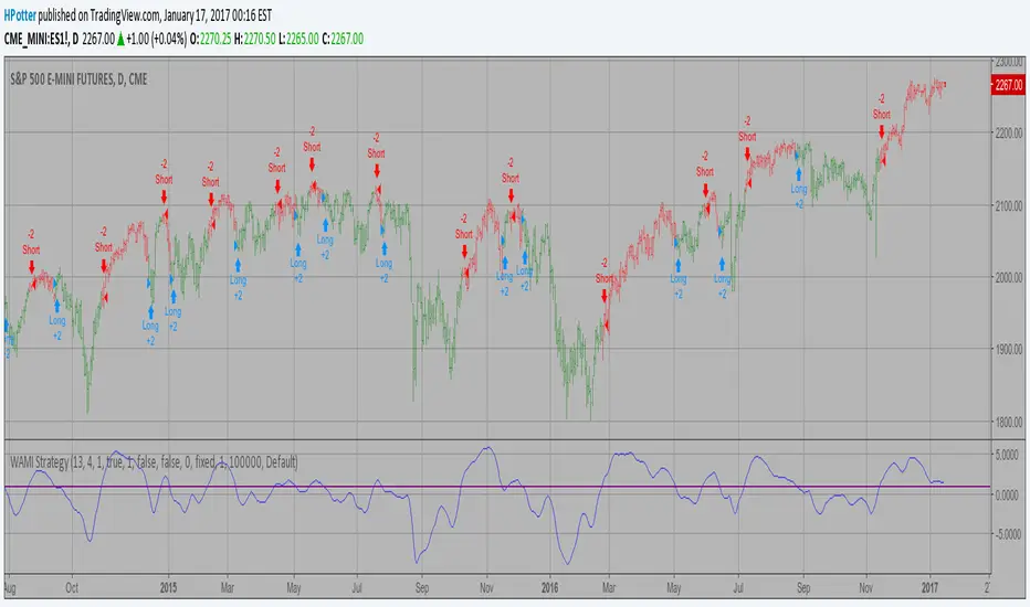
WAMI Strategy Backtest The WAMI-based trading lies in the application and iteration of the
optimization process until the indicated trades on past market data
give consistent, profitable results. It is rather difficult process
based on Fourier analysis.
You can to change Trigger parameter for to get best values of strategy.
You can change long to short in the Input Settings
Please, use it only for learning or paper trading. Do not for real trading.