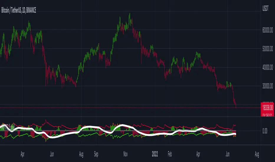
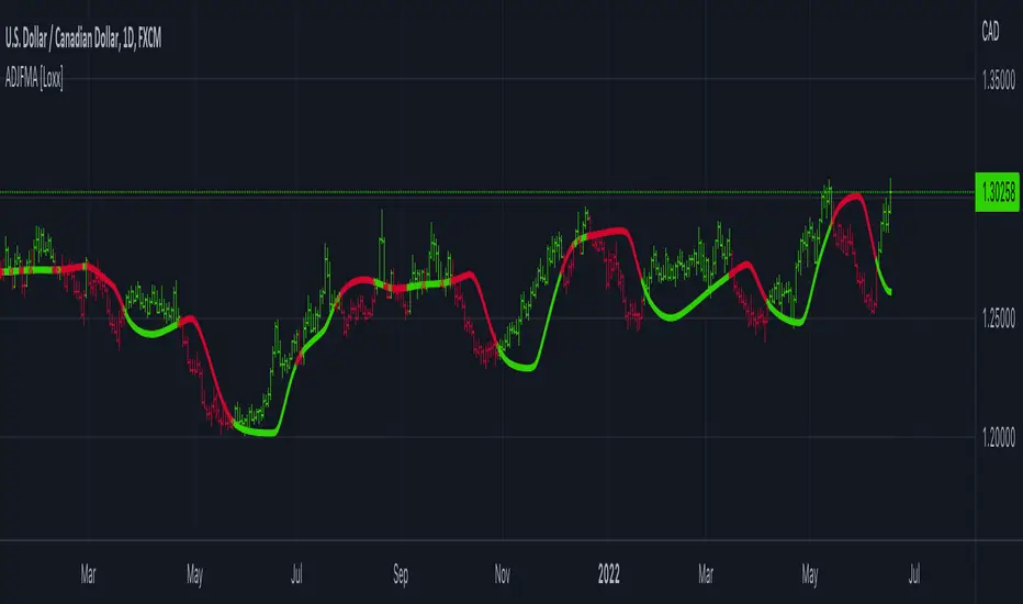
Adaptive, Jurik-Filtered, JMA/DWMA MACD [Loxx]Adaptive, Jurik-Filtered, JMA/DWMA MACD is MACD oscillator with a twist. The traditional calculation of MACD is the between two EMAs of price. This traditional approach yields a very noisy and lagged signal. To solve this problem, JMA/DWMA MACD uses the difference between adaptive Juirk-Filtered price and adaptive DWMA to yield a marked improvement over traditional MACD.
What is JMA / DWMA oscillator (MACD)?
Of all the different combinations of moving average filters to use for a MACD oscillator, we prefer using the JMA - DWMA combination.
JMA is ideal for the fast moving average line because it is quick to respond to reversals, is smooth and can be set to have no overshoot. DWMA (double weighted moving average) is ideal for the slower line as is tends to delay reversing direction until JMA crosses it.
What is Jurik Volty used in the Juirk Filter?
One of the lesser known qualities of Juirk smoothing is that the Jurik smoothing process is adaptive. "Jurik Volty" (a sort of market volatility ) is what makes Jurik smoothing adaptive. The Jurik Volty calculation can be used as both a standalone indicator and to smooth other indicators that you wish to make adaptive.
What is the Jurik Moving Average?
Have you noticed how moving averages add some lag (delay) to your signals? ... especially when price gaps up or down in a big move, and you are waiting for your moving average to catch up? Wait no more! JMA eliminates this problem forever and gives you the best of both worlds: low lag and smooth lines.
Ideally, you would like a filtered signal to be both smooth and lag-free. Lag causes delays in your trades, and increasing lag in your indicators typically result in lower profits. In other words, late comers get what's left on the table after the feast has already begun.
What is an adaptive cycle, and what is Ehlers Autocorrelation Periodogram Algorithm?
From his Ehlers' book Cycle Analytics for Traders Advanced Technical Trading Concepts by John F. Ehlers , 2013, page 135:
"Adaptive filters can have several different meanings. For example, Perry Kaufman’s adaptive moving average ( KAMA ) and Tushar Chande’s variable index dynamic average ( VIDYA ) adapt to changes in volatility . By definition, these filters are reactive to price changes, and therefore they close the barn door after the horse is gone.The adaptive filters discussed in this chapter are the familiar Stochastic , relative strength index ( RSI ), commodity channel index ( CCI ), and band-pass filter.The key parameter in each case is the look-back period used to calculate the indicator. This look-back period is commonly a fixed value. However, since the measured cycle period is changing, it makes sense to adapt these indicators to the measured cycle period. When tradable market cycles are observed, they tend to persist for a short while.Therefore, by tuning the indicators to the measure cycle period they are optimized for current conditions and can even have predictive characteristics.
The dominant cycle period is measured using the Autocorrelation Periodogram Algorithm. That dominant cycle dynamically sets the look-back period for the indicators. I employ my own streamlined computation for the indicators that provide smoother and easier to interpret outputs than traditional methods. Further, the indicator codes have been modified to remove the effects of spectral dilation.This basically creates a whole new set of indicators for your trading arsenal."
Included
- Toggle on/off bar coloring
Ehlers

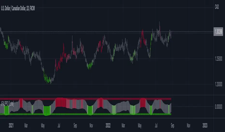
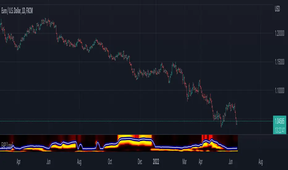
Jurik-Filtered, Adaptive Laguerre PPO [Loxx]Jurik-Filtered, Adaptive Laguerre PPO is an indicator used to find reversals. Smoothing with a Jurik Filter reduces noise and better identifies reversal points.
What is Laguerre Filter?
The Adaptive Laguerre is based on the Laguerre filter, described by John Ehlers in his paper “Time Warp – Without Space Travel”. It applies a variable gamma factor, based on how well the filter is tracking previous price movement. As with other adaptive moving averages, the Adaptive Laguerre tracks trending markets closely but will see less changes in range-bound markets.
The Adaptive Laguerre filter allows for an adjustment of the simple Laguerre filter. When price moves away from the filter, it becomes faster. When price moves sideward, the filter gets slower. Accordingly, this indicator belongs to the same class of moving average as the Kaufman Adaptive Moving Average (KAMA). It similar to the Volatility Index Dynamic Average (VIDYA) developed by Tushar Chande. The Adaptive Laguerre filter is smoother than the VIDYA and will adjust slower to price action after consolidations.
What is Jurik Volty?
One of the lesser known qualities of Juirk smoothing is that the Jurik smoothing process is adaptive. "Jurik Volty" (a sort of market volatility ) is what makes Jurik smoothing adaptive. The Jurik Volty calculation can be used as both a standalone indicator and to smooth other indicators that you wish to make adaptive.
What is the Jurik Moving Average?
Have you noticed how moving averages add some lag (delay) to your signals? ... especially when price gaps up or down in a big move, and you are waiting for your moving average to catch up? Wait no more! JMA eliminates this problem forever and gives you the best of both worlds: low lag and smooth lines.
Ideally, you would like a filtered signal to be both smooth and lag-free. Lag causes delays in your trades, and increasing lag in your indicators typically result in lower profits. In other words, late comers get what's left on the table after the feast has already begun.
Included:
-Toggle on/off bar coloring
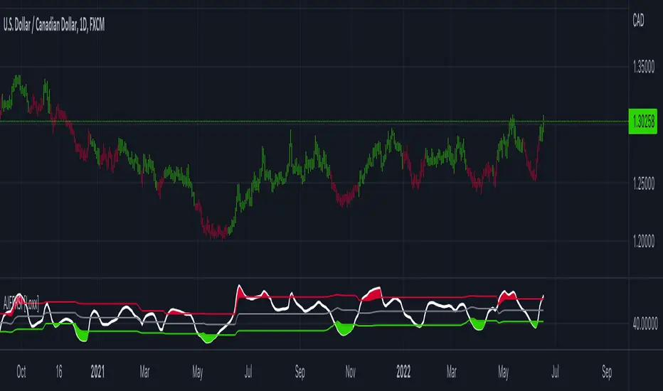
Adaptive, Jurik-Filtered, Floating RSI [Loxx]Adaptive, Jurik-Filtered, Floating RSI is an adaptive RSI indicator that smooths the RSI signal with a Jurik Filter.
This indicator contains three different types of RSI. They are following.
Wilders' RSI:
The Relative Strength Index ( RSI ) is a well versed momentum based oscillator which is used to measure the speed (velocity) as well as the change (magnitude) of directional price movements. Essentially RSI , when graphed, provides a visual mean to monitor both the current, as well as historical, strength and weakness of a particular market. The strength or weakness is based on closing prices over the duration of a specified trading period creating a reliable metric of price and momentum changes. Given the popularity of cash settled instruments (stock indexes) and leveraged financial products (the entire field of derivatives); RSI has proven to be a viable indicator of price movements.
RSX RSI:
RSI is a very popular technical indicator, because it takes into consideration market speed, direction and trend uniformity. However, the its widely criticized drawback is its noisy (jittery) appearance. The Jurk RSX retains all the useful features of RSI , but with one important exception: the noise is gone with no added lag.
Rapid RSI:
Rapid RSI Indicator, from Ian Copsey's article in the October 2006 issue of Stocks & Commodities magazine.
RapidRSI resembles Wilder's RSI , but uses a SMA instead of a WilderMA for internal smoothing of price change accumulators.
This indicator also uses adaptive cycles to calculate input lengths
What is an adaptive cycle, and what is Ehlers Autocorrelation Periodogram Algorithm?
From his Ehlers' book Cycle Analytics for Traders Advanced Technical Trading Concepts by John F. Ehlers , 2013, page 135:
"Adaptive filters can have several different meanings. For example, Perry Kaufman’s adaptive moving average ( KAMA ) and Tushar Chande’s variable index dynamic average ( VIDYA ) adapt to changes in volatility . By definition, these filters are reactive to price changes, and therefore they close the barn door after the horse is gone.The adaptive filters discussed in this chapter are the familiar Stochastic , relative strength index ( RSI ), commodity channel index ( CCI ), and band-pass filter.The key parameter in each case is the look-back period used to calculate the indicator. This look-back period is commonly a fixed value. However, since the measured cycle period is changing, it makes sense to adapt these indicators to the measured cycle period. When tradable market cycles are observed, they tend to persist for a short while.Therefore, by tuning the indicators to the measure cycle period they are optimized for current conditions and can even have predictive characteristics.
The dominant cycle period is measured using the Autocorrelation Periodogram Algorithm. That dominant cycle dynamically sets the look-back period for the indicators. I employ my own streamlined computation for the indicators that provide smoother and easier to interpret outputs than traditional methods. Further, the indicator codes have been modified to remove the effects of spectral dilation.This basically creates a whole new set of indicators for your trading arsenal."
Lastly, RSI is filtered and smoothed using a Jurik Filter
What is Jurik Volty?
One of the lesser known qualities of Juirk smoothing is that the Jurik smoothing process is adaptive. "Jurik Volty" (a sort of market volatility ) is what makes Jurik smoothing adaptive. The Jurik Volty calculation can be used as both a standalone indicator and to smooth other indicators that you wish to make adaptive.
What is the Jurik Moving Average?
Have you noticed how moving averages add some lag (delay) to your signals? ... especially when price gaps up or down in a big move, and you are waiting for your moving average to catch up? Wait no more! JMA eliminates this problem forever and gives you the best of both worlds: low lag and smooth lines.
Ideally, you would like a filtered signal to be both smooth and lag-free. Lag causes delays in your trades, and increasing lag in your indicators typically result in lower profits. In other words, late comers get what's left on the table after the feast has already begun.
Usage
-Red fill color when RSI is in overbought zone means a possible bear trend is incoming
-Green fill color when RSI is in overbought zone means a possible bear trend is incoming
Included
-Bar coloring
Adaptive Jurik Filter MACD [Loxx]Adaptive Jurik Filter MACD uses Jurik Volty and Adaptive Double Jurik Filter Moving Average (AJFMA) to derive Jurik Filter smoothed volatility.
What is MACD?
Moving average convergence divergence (MACD) is a trend-following momentum indicator that shows the relationship between two moving averages of a security’s price. The MACD is calculated by subtracting the 26-period exponential moving average (EMA) from the 12-period EMA.
The result of that calculation is the MACD line. A nine-day EMA of the MACD called the "signal line," is then plotted on top of the MACD line, which can function as a trigger for buy and sell signals. Traders may buy the security when the MACD crosses above its signal line and sell—or short—the security when the MACD crosses below the signal line. Moving average convergence divergence (MACD) indicators can be interpreted in several ways, but the more common methods are crossovers, divergences, and rapid rises/falls.
What is Jurik Volty?
One of the lesser known qualities of Juirk smoothing is that the Jurik smoothing process is adaptive. "Jurik Volty" (a sort of market volatility ) is what makes Jurik smoothing adaptive. The Jurik Volty calculation can be used as both a standalone indicator and to smooth other indicators that you wish to make adaptive.
What is the Jurik Moving Average?
Have you noticed how moving averages add some lag (delay) to your signals? ... especially when price gaps up or down in a big move, and you are waiting for your moving average to catch up? Wait no more! JMA eliminates this problem forever and gives you the best of both worlds: low lag and smooth lines.
Ideally, you would like a filtered signal to be both smooth and lag-free. Lag causes delays in your trades, and increasing lag in your indicators typically result in lower profits. In other words, late comers get what's left on the table after the feast has already begun.
That's why investors, banks and institutions worldwide ask for the Jurik Research Moving Average ( JMA ). You may apply it just as you would any other popular moving average. However, JMA's improved timing and smoothness will astound you.
What is adaptive Jurik volatility?
One of the lesser known qualities of Juirk smoothing is that the Jurik smoothing process is adaptive. "Jurik Volty" (a sort of market volatility ) is what makes Jurik smoothing adaptive. The Jurik Volty calculation can be used as both a standalone indicator and to smooth other indicators that you wish to make adaptive.
What is an adaptive cycle, and what is Ehlers Autocorrelation Periodogram Algorithm?
From his Ehlers' book Cycle Analytics for Traders Advanced Technical Trading Concepts by John F. Ehlers , 2013, page 135:
"Adaptive filters can have several different meanings. For example, Perry Kaufman’s adaptive moving average ( KAMA ) and Tushar Chande’s variable index dynamic average ( VIDYA ) adapt to changes in volatility . By definition, these filters are reactive to price changes, and therefore they close the barn door after the horse is gone.The adaptive filters discussed in this chapter are the familiar Stochastic , relative strength index ( RSI ), commodity channel index ( CCI ), and band-pass filter.The key parameter in each case is the look-back period used to calculate the indicator. This look-back period is commonly a fixed value. However, since the measured cycle period is changing, it makes sense to adapt these indicators to the measured cycle period. When tradable market cycles are observed, they tend to persist for a short while.Therefore, by tuning the indicators to the measure cycle period they are optimized for current conditions and can even have predictive characteristics.
The dominant cycle period is measured using the Autocorrelation Periodogram Algorithm. That dominant cycle dynamically sets the look-back period for the indicators. I employ my own streamlined computation for the indicators that provide smoother and easier to interpret outputs than traditional methods. Further, the indicator codes have been modified to remove the effects of spectral dilation.This basically creates a whole new set of indicators for your trading arsenal."
Included
- Change colors of oscillators and bars

Adaptive Jurik Filter Volatility Oscillator [Loxx]Adaptive Jurik Filter Volatility Oscillator uses Jurik Volty and Adaptive Double Jurik Filter Moving Average (AJFMA) to derive Jurik Filter smoothed volatility.
What is Jurik Volty?
One of the lesser known qualities of Juirk smoothing is that the Jurik smoothing process is adaptive. "Jurik Volty" (a sort of market volatility ) is what makes Jurik smoothing adaptive. The Jurik Volty calculation can be used as both a standalone indicator and to smooth other indicators that you wish to make adaptive.
What is the Jurik Moving Average?
Have you noticed how moving averages add some lag (delay) to your signals? ... especially when price gaps up or down in a big move, and you are waiting for your moving average to catch up? Wait no more! JMA eliminates this problem forever and gives you the best of both worlds: low lag and smooth lines.
Ideally, you would like a filtered signal to be both smooth and lag-free. Lag causes delays in your trades, and increasing lag in your indicators typically result in lower profits. In other words, late comers get what's left on the table after the feast has already begun.
That's why investors, banks and institutions worldwide ask for the Jurik Research Moving Average ( JMA ). You may apply it just as you would any other popular moving average. However, JMA's improved timing and smoothness will astound you.
What is adaptive Jurik volatility?
One of the lesser known qualities of Juirk smoothing is that the Jurik smoothing process is adaptive. "Jurik Volty" (a sort of market volatility ) is what makes Jurik smoothing adaptive. The Jurik Volty calculation can be used as both a standalone indicator and to smooth other indicators that you wish to make adaptive.
What is an adaptive cycle, and what is Ehlers Autocorrelation Periodogram Algorithm?
From his Ehlers' book Cycle Analytics for Traders Advanced Technical Trading Concepts by John F. Ehlers , 2013, page 135:
"Adaptive filters can have several different meanings. For example, Perry Kaufman’s adaptive moving average ( KAMA ) and Tushar Chande’s variable index dynamic average ( VIDYA ) adapt to changes in volatility . By definition, these filters are reactive to price changes, and therefore they close the barn door after the horse is gone.The adaptive filters discussed in this chapter are the familiar Stochastic , relative strength index ( RSI ), commodity channel index ( CCI ), and band-pass filter.The key parameter in each case is the look-back period used to calculate the indicator. This look-back period is commonly a fixed value. However, since the measured cycle period is changing, it makes sense to adapt these indicators to the measured cycle period. When tradable market cycles are observed, they tend to persist for a short while.Therefore, by tuning the indicators to the measure cycle period they are optimized for current conditions and can even have predictive characteristics.
The dominant cycle period is measured using the Autocorrelation Periodogram Algorithm. That dominant cycle dynamically sets the look-back period for the indicators. I employ my own streamlined computation for the indicators that provide smoother and easier to interpret outputs than traditional methods. Further, the indicator codes have been modified to remove the effects of spectral dilation.This basically creates a whole new set of indicators for your trading arsenal."
Included
- UI options to color bars
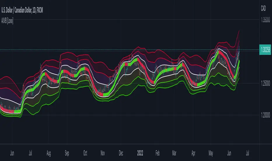
Adaptive Jurik Filter Volatility Bands [Loxx]Adaptive Jurik Filter Volatility Bands uses Jurik Volty and Adaptive, Double Jurik Filter Moving Average (AJFMA) to derive Jurik Filter smoothed volatility channels around an Adaptive Jurik Filter Moving Average. Bands are placed at 1, 2, and 3 deviations from the core basline.
What is Jurik Volty?
One of the lesser known qualities of Juirk smoothing is that the Jurik smoothing process is adaptive. "Jurik Volty" (a sort of market volatility ) is what makes Jurik smoothing adaptive. The Jurik Volty calculation can be used as both a standalone indicator and to smooth other indicators that you wish to make adaptive.
What is the Jurik Moving Average?
Have you noticed how moving averages add some lag (delay) to your signals? ... especially when price gaps up or down in a big move, and you are waiting for your moving average to catch up? Wait no more! JMA eliminates this problem forever and gives you the best of both worlds: low lag and smooth lines.
Ideally, you would like a filtered signal to be both smooth and lag-free. Lag causes delays in your trades, and increasing lag in your indicators typically result in lower profits. In other words, late comers get what's left on the table after the feast has already begun.
That's why investors, banks and institutions worldwide ask for the Jurik Research Moving Average ( JMA ). You may apply it just as you would any other popular moving average. However, JMA's improved timing and smoothness will astound you.
What is adaptive Jurik volatility?
One of the lesser known qualities of Juirk smoothing is that the Jurik smoothing process is adaptive. "Jurik Volty" (a sort of market volatility ) is what makes Jurik smoothing adaptive. The Jurik Volty calculation can be used as both a standalone indicator and to smooth other indicators that you wish to make adaptive.
What is an adaptive cycle, and what is Ehlers Autocorrelation Periodogram Algorithm?
From his Ehlers' book Cycle Analytics for Traders Advanced Technical Trading Concepts by John F. Ehlers , 2013, page 135:
"Adaptive filters can have several different meanings. For example, Perry Kaufman’s adaptive moving average ( KAMA ) and Tushar Chande’s variable index dynamic average ( VIDYA ) adapt to changes in volatility . By definition, these filters are reactive to price changes, and therefore they close the barn door after the horse is gone.The adaptive filters discussed in this chapter are the familiar Stochastic , relative strength index ( RSI ), commodity channel index ( CCI ), and band-pass filter.The key parameter in each case is the look-back period used to calculate the indicator. This look-back period is commonly a fixed value. However, since the measured cycle period is changing, it makes sense to adapt these indicators to the measured cycle period. When tradable market cycles are observed, they tend to persist for a short while.Therefore, by tuning the indicators to the measure cycle period they are optimized for current conditions and can even have predictive characteristics.
The dominant cycle period is measured using the Autocorrelation Periodogram Algorithm. That dominant cycle dynamically sets the look-back period for the indicators. I employ my own streamlined computation for the indicators that provide smoother and easier to interpret outputs than traditional methods. Further, the indicator codes have been modified to remove the effects of spectral dilation.This basically creates a whole new set of indicators for your trading arsenal."
Included
- UI options to shut off colors and bands
Adaptive, Double Jurik Filter Moving Average (AJFMA) [Loxx]Adaptive, Double Jurik Filter Moving Average (AJFMA) is moving average like Jurik Moving Average but with the addition of double smoothing and adaptive length (Autocorrelation Periodogram Algorithm) and power/volatility {Juirk Volty) inputs to further reduce noise and identify trends.
What is Jurik Volty?
One of the lesser known qualities of Juirk smoothing is that the Jurik smoothing process is adaptive. "Jurik Volty" (a sort of market volatility ) is what makes Jurik smoothing adaptive. The Jurik Volty calculation can be used as both a standalone indicator and to smooth other indicators that you wish to make adaptive.
What is the Jurik Moving Average?
Have you noticed how moving averages add some lag (delay) to your signals? ... especially when price gaps up or down in a big move, and you are waiting for your moving average to catch up? Wait no more! JMA eliminates this problem forever and gives you the best of both worlds: low lag and smooth lines.
Ideally, you would like a filtered signal to be both smooth and lag-free. Lag causes delays in your trades, and increasing lag in your indicators typically result in lower profits. In other words, late comers get what's left on the table after the feast has already begun.
That's why investors, banks and institutions worldwide ask for the Jurik Research Moving Average ( JMA ). You may apply it just as you would any other popular moving average. However, JMA's improved timing and smoothness will astound you.
What is adaptive Jurik volatility?
One of the lesser known qualities of Juirk smoothing is that the Jurik smoothing process is adaptive. "Jurik Volty" (a sort of market volatility ) is what makes Jurik smoothing adaptive. The Jurik Volty calculation can be used as both a standalone indicator and to smooth other indicators that you wish to make adaptive.
What is an adaptive cycle, and what is Ehlers Autocorrelation Periodogram Algorithm?
From his Ehlers' book Cycle Analytics for Traders Advanced Technical Trading Concepts by John F. Ehlers , 2013, page 135:
"Adaptive filters can have several different meanings. For example, Perry Kaufman’s adaptive moving average ( KAMA ) and Tushar Chande’s variable index dynamic average ( VIDYA ) adapt to changes in volatility . By definition, these filters are reactive to price changes, and therefore they close the barn door after the horse is gone.The adaptive filters discussed in this chapter are the familiar Stochastic , relative strength index ( RSI ), commodity channel index ( CCI ), and band-pass filter.The key parameter in each case is the look-back period used to calculate the indicator. This look-back period is commonly a fixed value. However, since the measured cycle period is changing, it makes sense to adapt these indicators to the measured cycle period. When tradable market cycles are observed, they tend to persist for a short while.Therefore, by tuning the indicators to the measure cycle period they are optimized for current conditions and can even have predictive characteristics.
The dominant cycle period is measured using the Autocorrelation Periodogram Algorithm. That dominant cycle dynamically sets the look-back period for the indicators. I employ my own streamlined computation for the indicators that provide smoother and easier to interpret outputs than traditional methods. Further, the indicator codes have been modified to remove the effects of spectral dilation.This basically creates a whole new set of indicators for your trading arsenal."
Included
- Double calculation of AJFMA for even smoother results
Adaptive, Jurik-Smoothed, Trend Continuation Factor [Loxx]Adaptive, Jurik-Smoothed, Trend Continuation Factor is a Trend Continuation Factor indicator with adaptive length and volatility inputs
What is the Trend Continuation Factor?
The Trend Continuation Factor (TCF) identifies the trend and its direction. TCF was introduced by M. H. Pee. Positive values of either the Positive Trend Continuation Factor (TCF+) and the Negative Trend Continuation Factor (TCF-) indicate the presence of a strong trend.
What is the Jurik Moving Average?
Have you noticed how moving averages add some lag (delay) to your signals? ... especially when price gaps up or down in a big move, and you are waiting for your moving average to catch up? Wait no more! JMA eliminates this problem forever and gives you the best of both worlds: low lag and smooth lines.
Ideally, you would like a filtered signal to be both smooth and lag-free. Lag causes delays in your trades, and increasing lag in your indicators typically result in lower profits. In other words, late comers get what's left on the table after the feast has already begun.
That's why investors, banks and institutions worldwide ask for the Jurik Research Moving Average ( JMA ). You may apply it just as you would any other popular moving average. However, JMA's improved timing and smoothness will astound you.
What is adaptive Jurik volatility?
One of the lesser known qualities of Juirk smoothing is that the Jurik smoothing process is adaptive. "Jurik Volty" (a sort of market volatility ) is what makes Jurik smoothing adaptive. The Jurik Volty calculation can be used as both a standalone indicator and to smooth other indicators that you wish to make adaptive.
What is an adaptive cycle, and what is Ehlers Autocorrelation Periodogram Algorithm?
From his Ehlers' book Cycle Analytics for Traders Advanced Technical Trading Concepts by John F. Ehlers , 2013, page 135:
"Adaptive filters can have several different meanings. For example, Perry Kaufman’s adaptive moving average ( KAMA ) and Tushar Chande’s variable index dynamic average ( VIDYA ) adapt to changes in volatility . By definition, these filters are reactive to price changes, and therefore they close the barn door after the horse is gone.The adaptive filters discussed in this chapter are the familiar Stochastic , relative strength index ( RSI ), commodity channel index ( CCI ), and band-pass filter.The key parameter in each case is the look-back period used to calculate the indicator. This look-back period is commonly a fixed value. However, since the measured cycle period is changing, it makes sense to adapt these indicators to the measured cycle period. When tradable market cycles are observed, they tend to persist for a short while.Therefore, by tuning the indicators to the measure cycle period they are optimized for current conditions and can even have predictive characteristics.
The dominant cycle period is measured using the Autocorrelation Periodogram Algorithm. That dominant cycle dynamically sets the look-back period for the indicators. I employ my own streamlined computation for the indicators that provide smoother and easier to interpret outputs than traditional methods. Further, the indicator codes have been modified to remove the effects of spectral dilation.This basically creates a whole new set of indicators for your trading arsenal."
Included
-Your choice of length input calculation, either fixed or adaptive cycle
-Bar coloring to paint the trend
Happy trading!

TASC 2022.07 Pairs Rotation With Ehlers Loops█ OVERVIEW
TASC's July 2022 edition of Traders' Tips includes an article by John Ehlers titled "Pairs Rotation With Ehlers Loops". This is the code that implements the Ehlers Loops applied to pairs rotation trading.
█ CONCEPTS
John Ehlers developed Ehlers loops as a tool to visualize the performance of one data stream versus another. Initially, he used this tool to chart price versus volume. However, Ehlers loops proved to be suitable for determining the timing of the pairs rotation strategy . This strategy works by having a long position in only one of two securities, depending on which one is considered stronger at a given time.
When the prices of two securities (filtered and scaled with a standard deviation for consistent presentation) are plotted against each other, the curvature and direction of rotation on the chart can help guide decisions on long positions. For example, when plotting a stock versus a referenced symbol, a vertical upward movement while rotating clockwise is a sign of going long the stock. Similarly, a horizontal movement to the right while rotating counterclockwise is the sign to go long the reference. A higher probability of a reversal is expected when the price moves more than one or two standard deviations.
█ CALCULATIONS
The script uses the following steps to calculate the Ehlers Loops:
The price data of both securities in the pair are individually filtered using identical high-pass and SuperSmoother filters. This results in two band-limited data streams, having a nominally zero mean. The input parameters Low-Pass Period and High-Pass Period control the filter bandwidth and thus can modify the shape of the Ehlers Loops.
Subsequently, the filtered data streams are scaled in terms of standard deviation by dividing each of them by their root-mean-square (RMS) values. These data streams are plotted as zero-mean oscillators.
Finally, the scaled data streams are displayed one against another for the selected time interval (defined by the input parameter Loop Segments ). In the resulting scatterplot, the thicker line corresponds to the later data points. The fluctuations of the filtered price data of the chart symbol are plotted along the y -axis, and the price changes of the referenced symbol are shown along the x -axis.

Ehlers Autocorrelation Periodogram [Loxx]Ehlers Autocorrelation Periodogram contains two versions of Ehlers Autocorrelation Periodogram Algorithm. This indicator is meant to supplement adaptive cycle indicators that myself and others have published on Trading View, will continue to publish on Trading View. These are fast-loading, low-overhead, streamlined, exact replicas of Ehlers' work without any other adjustments or inputs.
Versions:
- 2013, Cycle Analytics for Traders Advanced Technical Trading Concepts by John F. Ehlers
- 2016, TASC September, "Measuring Market Cycles"
Description
The Ehlers Autocorrelation study is a technical indicator used in the calculation of John F. Ehlers’s Autocorrelation Periodogram. Its main purpose is to eliminate noise from the price data, reduce effects of the “spectral dilation” phenomenon, and reveal dominant cycle periods. The spectral dilation has been discussed in several studies by John F. Ehlers; for more information on this, refer to sources in the "Further Reading" section.
As the first step, Autocorrelation uses Mr. Ehlers’s previous installment, Ehlers Roofing Filter, in order to enhance the signal-to-noise ratio and neutralize the spectral dilation. This filter is based on aerospace analog filters and when applied to market data, it attempts to only pass spectral components whose periods are between 10 and 48 bars.
Autocorrelation is then applied to the filtered data: as its name implies, this function correlates the data with itself a certain period back. As with other correlation techniques, the value of +1 would signify the perfect correlation and -1, the perfect anti-correlation.
Using values of Autocorrelation in Thermo Mode may help you reveal the cycle periods within which the data is best correlated (or anti-correlated) with itself. Those periods are displayed in the extreme colors (orange) while areas of intermediate colors mark periods of less useful cycles.
What is an adaptive cycle, and what is the Autocorrelation Periodogram Algorithm?
From his Ehlers' book mentioned above, page 135:
"Adaptive filters can have several different meanings. For example, Perry Kaufman’s adaptive moving average ( KAMA ) and Tushar Chande’s variable index dynamic average ( VIDYA ) adapt to changes in volatility . By definition, these filters are reactive to price changes, and therefore they close the barn door after the horse is gone.The adaptive filters discussed in this chapter are the familiar Stochastic , relative strength index ( RSI ), commodity channel index ( CCI ), and band-pass filter.The key parameter in each case is the look-back period used to calculate the indicator.This look-back period is commonly a fixed value. However, since the measured cycle period is changing, as we have seen in previous chapters, it makes sense to adapt these indicators to the measured cycle period. When tradable market cycles are observed, they tend to persist for a short while.Therefore, by tuning the indicators to the measure cycle period they are optimized for current conditions and can even have predictive characteristics.
The dominant cycle period is measured using the Autocorrelation Periodogram Algorithm. That dominant cycle dynamically sets the look-back period for the indicators. I employ my own streamlined computation for the indicators that provide smoother and easier to interpret outputs than traditional methods. Further, the indicator codes have been modified to remove the effects of spectral dilation.This basically creates a whole new set of indicators for your trading arsenal."
How to use this indicator
The point of the Ehlers Autocorrelation Periodogram Algorithm is to dynamically set a period between a minimum and a maximum period length. While I leave the exact explanation of the mechanic to Dr. Ehlers’s book, for all practical intents and purposes, in my opinion, the punchline of this method is to attempt to remove a massive source of overfitting from trading system creation–namely specifying a look-back period. SMA of 50 days? 100 days? 200 days? Well, theoretically, this algorithm takes that possibility of overfitting out of your hands. Simply, specify an upper and lower bound for your look-back, and it does the rest. In addition, this indicator tells you when its best to use adaptive cycle inputs for your other indicators.
Usage Example 1
Let's say you're using "Adaptive Qualitative Quantitative Estimation (QQE) ". This indicator has the option of adaptive cycle inputs. When the "Ehlers Autocorrelation Periodogram " shows a period of high correlation that adaptive cycle inputs work best during that period.
Usage Example 2
Check where the dominant cycle line lines, grab that output number and inject it into your other standard indicators for the length input.
Ehlers Adaptive Relative Strength Index (RSI) [Loxx]Ehlers Adaptive Relative Strength Index (RSI) is an implementation of RSI using Ehlers Autocorrelation Periodogram Algorithm to derive the length input for RSI. Other implementations of Ehers Adaptive RSI rely on the inferior Hilbert Transformer derive the dominant cycle.
In his book "Cycle Analytics for Traders Advanced Technical Trading Concepts", John F. Ehlers describes an implementation for Adaptive Relative Strength Index in order to solve for varying length inputs into the classic RSI equation.
What is an adaptive cycle, and what is the Autocorrelation Periodogram Algorithm?
From his Ehlers' book mentioned above, page 135:
"Adaptive filters can have several different meanings. For example, Perry Kaufman’s adaptive moving average (KAMA) and Tushar Chande’s variable index dynamic average (VIDYA) adapt to changes in volatility. By definition, these filters are reactive to price changes, and therefore they close the barn door after the horse is gone.The adaptive filters discussed in this chapter are the familiar Stochastic, relative strength index (RSI), commodity channel index (CCI), and band-pass filter.The key parameter in each case is the look-back period used to calculate the indicator.This look-back period is commonly a fixed value. However, since the measured cycle period is changing, as we have seen in previous chapters, it makes sense to adapt these indicators to the measured cycle period. When tradable market cycles are observed, they tend to persist for a short while.Therefore, by tuning the indicators to the measure cycle period they are optimized for current conditions and can even have predictive characteristics.
The dominant cycle period is measured using the autocorrelation periodogram algorithm. That dominant cycle dynamically sets the look-back period for the indicators. I employ my own streamlined computation for the indicators that provide smoother and easier to interpret outputs than traditional methods. Further, the indicator codes have been modified to remove the effects of spectral dilation.This basically creates a whole new set of indicators for your trading arsenal."
What is Adaptive RSI?
From his Ehlers' book mentioned above, page 137:
"The adaptive RSI starts with the computation of the dominant cycle using the autocorrelation periodogram approach. Since the objective is to use only those frequency components passed by the roofing filter, the variable "filt" is used as a data input rather than closing prices. Rather than independently taking the averages of the numerator and denominator, I chose to perform smoothing on the ratio using the SuperSmoother filter. The coefficients for the SuperSmoother filters have previously been computed in the dominant cycle measurement part of the code."
Happy trading!

Adaptive, Zero lag Schaff Trend Cycle Backtest (Simple) [Loxx]Simple backtest for "Adaptive, Zero lag Schaff Trend Cycle" found here:
What this backtest includes:
-Customization of inputs for Schaff Trend Cycle calculation
-Take profit 1 (TP1), and Stop-loss (SL), calculated using standard RMA-smoothed true range
-Activation of TP1 after entry candle closes
-Zero-cross entry signal plots
-Longs and shorts
-Continuation longs and shorts
Happy trading!

Adaptive, Zero lag Schaff Trend Cycle [Loxx]TASC's March 2008 edition Traders' Tips includes an article by John Ehlers titled "Measuring Cycle Periods," and describes the use of bandpass filters to estimate the length, in bars, of the currently dominant price cycle.
What are Dominant Cycles and Why should we use them?
Even the most casual chart reader will be able to spot times when the market is cycling and other times when longer-term trends are in play. Cycling markets are ideal for swing trading however attempting to “trade the swing” in a trending market can be a recipe for disaster. Similarly, applying trend trading techniques during a cycling market can equally wreak havoc in your account. Cycle or trend modes can readily be identified in hindsight. But it would be useful to have an objective scientific approach to guide you as to the current market mode.
There are a number of tools already available to differentiate between cycle and trend modes. For example, measuring the trend slope over the cycle period to the amplitude of the cyclic swing is one possibility.
We begin by thinking of cycle mode in terms of frequency or its inverse, periodicity. Since the markets are fractal ; daily, weekly, and intraday charts are pretty much indistinguishable when time scales are removed. Thus it is useful to think of the cycle period in terms of its bar count. For example, a 20 bar cycle using daily data corresponds to a cycle period of approximately one month.
When viewed as a waveform, slow-varying price trends constitute the waveform's low frequency components and day-to-day fluctuations (noise) constitute the high frequency components. The objective in cycle mode is to filter out the unwanted components--both low frequency trends and the high frequency noise--and retain only the range of frequencies over the desired swing period. A filter for doing this is called a bandpass filter and the range of frequencies passed is the filter's bandwidth.
Indicator Features
-Zero lag or Regular Schaff Trend Cycle calculation
- Fixed or Band-pass Dominant Cycle for Schaff Trend Cycle MA period inputs
-10 different moving average options for Zero lag calculations
-Separate Band-pass Dominant Cycle calculations for both Schaff Trend Cycle and MA calculations
- Slow-to-Fast Band-pass Dominant Cycle input to tweak the ratio of Schaff Trend Cycle MA input periods as they relate to each other

Hybrid, Zero lag, Adaptive cycle MACD Backtest (Simple) [Loxx]Simple backtest for Hybrid, Zero lag, Adaptive cycle MACD Backtest (Simple) found here:
What this backtest includes:
-Customization of inputs for MACD calculation
-Take profit 1 (TP1), and Stop-loss (SL), calculated using standard RMA-smoothed true range
-Activation of TP1 after entry candle closes
-Zero-cross entry signal plots
-MACD-Signal cross entry continuations
-Longs and shorts
Happy trading!

Hybrid, Zero lag, Adaptive cycle MACD [Loxx]TASC's March 2008 edition Traders' Tips includes an article by John Ehlers titled "Measuring Cycle Periods," and describes the use of bandpass filters to estimate the length, in bars, of the currently dominant price cycle.
What are Dominant Cycles and Why should we use them?
Even the most casual chart reader will be able to spot times when the market is cycling and other times when longer-term trends are in play. Cycling markets are ideal for swing trading however attempting to “trade the swing” in a trending market can be a recipe for disaster. Similarly, applying trend trading techniques during a cycling market can equally wreak havoc in your account. Cycle or trend modes can readily be identified in hindsight. But it would be useful to have an objective scientific approach to guide you as to the current market mode.
There are a number of tools already available to differentiate between cycle and trend modes. For example, measuring the trend slope over the cycle period to the amplitude of the cyclic swing is one possibility.
We begin by thinking of cycle mode in terms of frequency or its inverse, periodicity. Since the markets are fractal; daily, weekly, and intraday charts are pretty much indistinguishable when time scales are removed. Thus it is useful to think of the cycle period in terms of its bar count. For example, a 20 bar cycle using daily data corresponds to a cycle period of approximately one month.
When viewed as a waveform, slow-varying price trends constitute the waveform's low frequency components and day-to-day fluctuations (noise) constitute the high frequency components. The objective in cycle mode is to filter out the unwanted components--both low frequency trends and the high frequency noise--and retain only the range of frequencies over the desired swing period. A filter for doing this is called a bandpass filter and the range of frequencies passed is the filter's bandwidth .
Indicator Features
-Zero lag or Regular MACD/signal calculation
- Fixed or Band-pass Dominant Cycle for MACD and Signal MA period inputs
-10 different moving average options for both MACD and Signal MA calculations
-Separate Band-pass Dominant Cycle calculations for both MACD and Signal MA calculations
- Slow-to-Fast Band-pass Dominant Cycle input to tweak the ratio of MACD MA input periods as they relate to each other

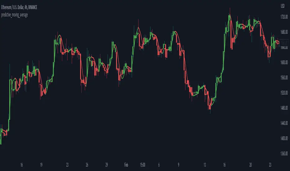
predictive_moving_average
Description:
Originated by John F. Ehlers, could be found within (Rocket Science for Traders, pg. 212). Aim to provide a leading indicator (I assumed for the shorter time period), which smoothed the price with no lag. The indicator derives from 2 lines crossing i.e. a weighted moving average, of higher length as a predictor and shorter length as a trigger.
Predictive Moving Average:
predict = 2*wma1 - wma2
trigger = (4*predict+3*predict +2*predict +predict)/10
Feature:
Predictive moving average
Deviation band
Notes
Consider the support/resistance (dynamic) when entering the position
Some short direction change might be identified from deviation shrink
Green indicates to enter/long, while red indicates to close/short position
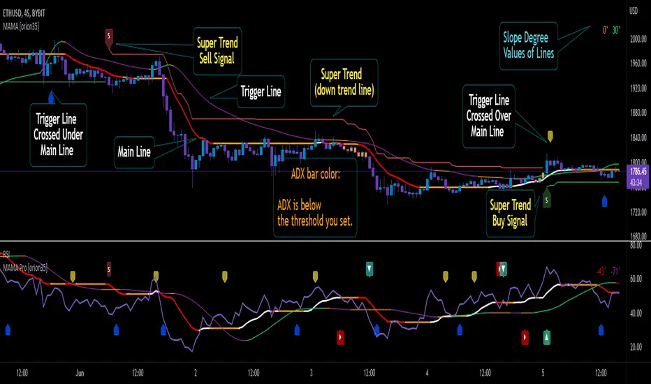
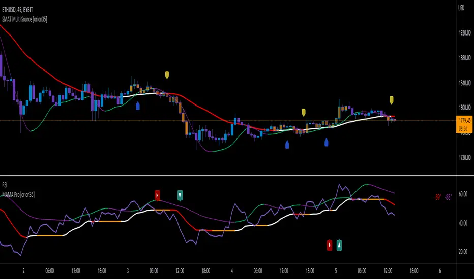
Mother of All Moving Averages, MAMA [orion35]This indicator contains the huge number of 53 MA tools . So, with the Mother of All Moving Averages (MAMA) , you can draw any two of these MA tools (that is, almost all the "Moving Average" tools used in the market) in the length and thickness you want.
These MA tools include traditional averages such as SMA , EMA , DEMA, as well as innovative averaging tools such as LFS (Laguerre Filter Smoother), LSMA (Least Square Moving Average), ZLSMA (Zerolag LSMA ) developed by @veryfid and SSMA (Super Smoothed Moving Average ) by John F. Ehlers .
Another great feature of this indicator is that signals can be filtered according to the instant ADX (Average Directional Movement indeX) value of the market. By using this filter, false signals in horizontal markets can be reduced. Also, with the threshold value setting in the ADX filter, calibration can be made for different assets and time frames when desired. In addition, you can color the price bars according to the ADX threshold value you set.
You can also automatically color these drawings in conditional formats as you wish.
If desired, the intersections of the plotted curves can be showed as signals. You can also set alarms for these intersections.
This indicator contains almost twice as many MA tools as the previous Super Moving Average Tools, SMAT indicator. For this reason, they are gathered in two main groups as " Traditional " and " New Generation " MA tools.
These MA tools are listed as follows:
--------- Mostly Traditional MA Tool s ---------
LFS : Laguerre Filter Smoother
SMA : Simple Moving Average
EMA : Exponential MA
DEMA : Double EMA
TEMA : Triple EMA
QEMA : Quadrupole EMA @everget
ZLEMA : Zerolag EMA
KZLEMA : Kalman ZLEMA
LRSMA : Linear Regression SMA
LREMA : Linear Regression EMA
TMA : Triangular MA (slow)
TMA v2 : Triangular MA (normal)
TMA v3 : Triangular MA (fast) @Daveatt
SMMA : SMoothed MA
SSMA : Super Smoother MA © 2013 John F. Ehlers
SSF : Super Smoother Filter @DonovanWall
SSeMA : Smoothed SEnsitive MA @BakwaasTrading
WMA : Weighted MA
VWMA : Volume Weighted MA
VWAP : Volume Weighted Average Price
AMA : Adaptive MA @everget
KAMA : Kaufman's Adaptive MA
FrAMA : Fractal Adaptive MA @Shizaru
ALMA : Arnaud Legoux MA
--------- New Generation MA Tools ---------
HMA : Hull MA
EHMA : Exponential HMA @DonovanWall
JMA : Jurik MA @everget
RMA : Relative MA aka Rolling MA
LWMA : Linearly Weighted MA @io72signals
LSMA : Least Square MA
ZLSMA : Zerolag LSMA @veryfid
ARSI : Adaptive Relative Strength Index @everget
WWMA : Welles Wilder's MA @KivancOzbilgic
VMA : Variable MA by Tushar S. Chande,
VIDYA : Variable Index Dynamic Average @KivancOzbilgic
VIDYA v2 : @Mohamed3nan
TSF : True Strength Force @KivancOzbilgic
TILL : Tillson T3 MA @KivancOzbilgic
DAF : Dynamically Adjustable Filter @alexgrover
KFS : Kalman Filter Smoother @alexgrover
PKF : Parametric Kalman Filter @alexgrover
VAMA : Volatility Adjusted MA @Duyck
CTI : Correlation Trend Indicator by John Ehlers
BF : Blackman Filter @alexgrover
MAMA : MESA Adaptive MA aka: Mother of AMA @KivancOzbilgic
FAMA : Following Adaptive MA @KivancOzbilgic
ARMA : Autonomous Recursive MA @alexgrover
ZARMA : Zerolag ARMA @alexgrover
A2RMA : Adaptive ARMA @alexgrover
EDMA : Exponentially Deviating MA @MightyZinger
BLP : Butterworth Low Pass Filter @DonovanWall
GLP : Gaussian Low Pass Filter @DonovanWall
SWMA : Sine Weighted MA @blackcat1402
TASC 2022.06 Ehlers Loops█ OVERVIEW
TASC's June 2022 edition Traders' Tips includes an article by John Ehlers titled "Ehlers Loops. Part 1". This is the code implementing the price-volume Ehlers Loops he introduced in the publication.
█ CONCEPTS
John Ehlers developed Ehlers loops as a tool to visualize the performance of one data stream versus another, both filtered and scaled. In this article, the author applies his concept to exploit and/or dispel the dogmatic principles of reliable price-volume relationships.
The script offers two different ways to visualize Ehlers Loops:
Oscillators (default option)
In this implementation, filtered and scaled volume is plotted along with filtered and scaled price as zero-mean oscillators. Observation of the relative direction of volume and price oscillators can be discretionarily used to interpret and predict market conditions. For example, it is generally assumed that an increase in volume and an increase in price define a bullish condition. Similarly, decreasing volume and increasing price are generally considered bearish. A decrease in volume and a decrease in price is considered a bullish condition. The increase in volume and decrease in price is often thought to be bearish.
Scatterplot
This Crocker-style visualization displays filtered and scaled price against filtered and scaled volume for the selected timespan. Fluctuations in volume are plotted along the x -axis, while price changes along the y -axis. This way of visualizing the Ehlers Loop allows you to analyze the curvature and directional path of the price in relation to volume, offering a different comparative perspective. The boundaries of the price and volume scale on the Ehlers Loop Crocker-chart are presented in standard deviations. Deviations can be used to predict possible future price or volume fluctuations. The expected probability of potential reversals is 68%, 95% and 99.7% at one, two and three standard deviations, respectively.
█ CALCULATIONS
The following steps are used to build an Ehlers Loop:
• Both price and volume are filtered to be band-limited signals. This is done by applying the high-pass Butterworth filter in combination with the low-pass SuperSmooth filter.
The cutoff wavelengths of the high-pass and low-pass filters are defined by the input parameters HPPeriod and LPPeriod , respectively.
These values change the appearance of the Ehlers Loops and can be customized to your trading style.
• The filtered price and volume time series are then scaled in terms of standard deviation by dividing each by their root-mean-square values.
• The resultant price and volume data are plotted as zero-mean oscillators or as a scatterplot.

COG SSMACD COL combo with ADX Filter [orion35]This indicator consists of a combination of indicators produced by the most valuable developers in the market.
These are: Center of Gravity (COG) and Super Smoothed MACD (SSMACD) shared by @KivancOzbilgic and Center of Linearity (COL) shared by @alexgrover
I produced this indicator by writing new conditions that compare the signals given by these indicators with each other. I re-coded the change in the thickness of the cloud from the COL indicator as the middle horizontal line with varying color intensity and type. I have provided options for switching between these three indicators when desired.
Note: The strongest signals in the indicator are the blue colored triangles. Moderately strong ones are yellow signals. White colored signals are considered as the weakest signals.
Some minor fixes:
Some confusing words were thrown in the alarms section,
Added new alarm codes for any Triple or Double signals.
Major changes have been made with this update.
It is very important to know the direction and strength of the trend in financial markets. Therefore, ADX (Average Directional movement index) was developed by J. Welles Wilder in 1978 as an indicator of the trend strength in the prices of a financial instrument.
Especially in sideways markets, most indicators produce many false signals. However, these signals can be filtered with the ADX indicator. The price is considered sideways when the ADX is less than 20 as the threshold value.
With this update,
ADX filter can be activated when desired, and signals can be filtered flexibly according to the "threshold" value determined by the user. When the ADX filter is active, it will also reflect on the alarm conditions. Therefore, if an alarm is to be set according to the ADX filter, the filter must be activated first.
The colors of the lines and signals have been made changeable.
The visual level and thickness of the COL line has been made adjustable.
With this update, signals can be filtered according to the MavilimW indicator developed by @KivancOzbilgic
Filter Methods:
Normal: If the price is below the BlueW line, "bull" signals are filtered out, and above "bear" signals are filtered out.
Reverse : Applies the opposite of the normal method.
Fixed some visual bugs in switching between indicators.

Super Moving Average Tools [orion35]
This indicator has been developed to cover almost all types of moving averages (MA) used in the market. Two of the 21 MA tools can be drawn independently on the price chart.
These MA tools include traditional averages such as SMA , EMA , DEMA , as well as innovative averaging tools such as LFS (Laguerre Filter Smoother), LSMA (Least Square Moving Average), ZLSMA (Zerolag LSMA ) developed by @veryfid and SSMA (Super Smoothed Moving Average ) by John F. Ehlers .
In addition, the traditional bar opening or closing values can be drawn on the chart as a source, as well as the data produced by a different indicator (for example, RSI ) can be used to calculate the average with this indicator and can be plotted on that oscillator. The chart above shows the drawings made on both the price bars and the RSI oscillator.
If desired, the intersections of the plotted curves can be showed as signals. Also, alarms have been added according to the intersection conditions.
Another great feature of this indicator is that signals can be filtered according to the instant ADX (Average Directional Movement indeX) value of the market. By using this filter, false signals in horizontal markets can be reduced . Also, with the threshold value setting in the ADX filter, calibration can be made for different assets and time frames when desired.
In addition, when desired, the data of different indicators drawn by using the "Raw Source" option can be intersected.
You can also write the combinations you like from the different MA tools and settings you use as a comment below.
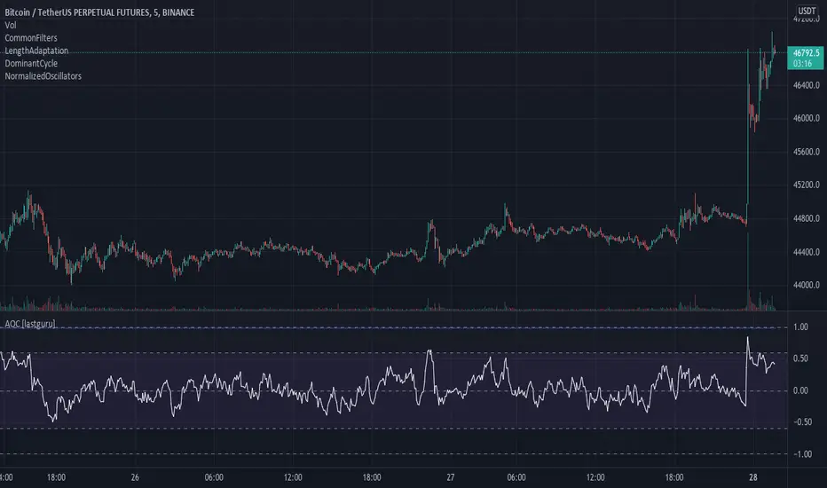
Adaptive MA Difference constructor [lastguru]A complimentary indicator to my Adaptive MA constructor. It calculates the difference between the two MA lines (inspired by the Moving Average Difference (MAD) indicator by John F. Ehlers). You can then further smooth the resulting curve. The parameters and options are explained here:
The difference is normalized by dividing the difference by twice its Root mean square (RMS) over Slow MA length. Inverse Fisher Transform is then used to force the -1..1 range.
Same Postfilter options are provided as in my Adaptive Oscillator constructor:
Stochastic - Stochastic
Super Smooth Stochastic - Super Smooth Stochastic (part of MESA Stochastic ) by John F. Ehlers
Inverse Fisher Transform - Inverse Fisher Transform
Noise Elimination Technology - a simplified Kendall correlation algorithm "Noise Elimination Technology" by John F. Ehlers
Momentum - momentum (derivative)
Except for Inverse Fisher Transform, all Postfilter algorithms can have Length parameter. If it is not specified (set to 0), then the calculated Slow MA Length is used.
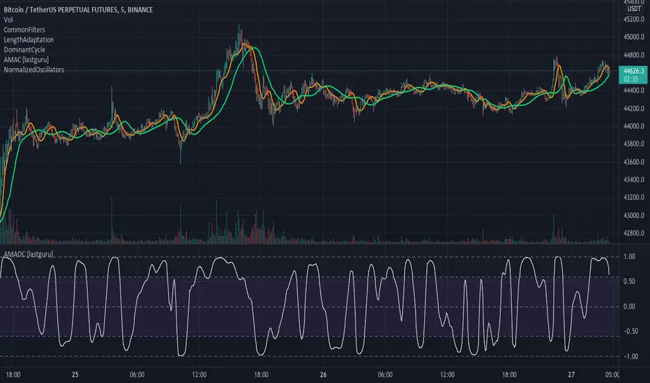
Adaptive Oscillator constructor [lastguru]Adaptive Oscillators use the same principle as Adaptive Moving Averages. This is an experiment to separate length generation from oscillators, offering multiple alternatives to be combined. Some of the combinations are widely known, some are not. Note that all Oscillators here are normalized to -1..1 range. This indicator is based on my previously published public libraries and also serve as a usage demonstration for them. I will try to expand the collection (suggestions are welcome), however it is not meant as an encyclopaedic resource , so you are encouraged to experiment yourself: by looking on the source code of this indicator, I am sure you will see how trivial it is to use the provided libraries and expand them with your own ideas and combinations. I give no recommendation on what settings to use, but if you find some useful setting, combination or application ideas (or bugs in my code), I would be happy to read about them in the comments section.
The indicator works in three stages: Prefiltering, Length Adaptation and Oscillators.
Prefiltering is a fast smoothing to get rid of high-frequency (2, 3 or 4 bar) noise.
Adaptation algorithms are roughly subdivided in two categories: classic Length Adaptations and Cycle Estimators (they are also implemented in separate libraries), all are selected in Adaptation dropdown. Length Adaptation used in the Adaptive Moving Averages and the Adaptive Oscillators try to follow price movements and accelerate/decelerate accordingly (usually quite rapidly with a huge range). Cycle Estimators, on the other hand, try to measure the cycle period of the current market, which does not reflect price movement or the rate of change (the rate of change may also differ depending on the cycle phase, but the cycle period itself usually changes slowly).
Chande (Price) - based on Chande's Dynamic Momentum Index (CDMI or DYMOI), which is dynamic RSI with this length
Chande (Volume) - a variant of Chande's algorithm, where volume is used instead of price
VIDYA - based on VIDYA algorithm. The period oscillates from the Lower Bound up (slow)
VIDYA-RS - based on Vitali Apirine's modification of VIDYA algorithm (he calls it Relative Strength Moving Average). The period oscillates from the Upper Bound down (fast)
Kaufman Efficiency Scaling - based on Efficiency Ratio calculation originally used in KAMA
Deviation Scaling - based on DSSS by John F. Ehlers
Median Average - based on Median Average Adaptive Filter by John F. Ehlers
Fractal Adaptation - based on FRAMA by John F. Ehlers
MESA MAMA Alpha - based on MESA Adaptive Moving Average by John F. Ehlers
MESA MAMA Cycle - based on MESA Adaptive Moving Average by John F. Ehlers , but unlike Alpha calculation, this adaptation estimates cycle period
Pearson Autocorrelation* - based on Pearson Autocorrelation Periodogram by John F. Ehlers
DFT Cycle* - based on Discrete Fourier Transform Spectrum estimator by John F. Ehlers
Phase Accumulation* - based on Dominant Cycle from Phase Accumulation by John F. Ehlers
Length Adaptation usually take two parameters: Bound From (lower bound) and To (upper bound). These are the limits for Adaptation values. Note that the Cycle Estimators marked with asterisks(*) are very computationally intensive, so the bounds should not be set much higher than 50, otherwise you may receive a timeout error (also, it does not seem to be a useful thing to do, but you may correct me if I'm wrong).
The Cycle Estimators marked with asterisks(*) also have 3 checkboxes: HP (Highpass Filter), SS (Super Smoother) and HW (Hann Window). These enable or disable their internal prefilters, which are recommended by their author - John F. Ehlers . I do not know, which combination works best, so you can experiment.
Chande's Adaptations also have 3 additional parameters: SD Length (lookback length of Standard deviation), Smooth (smoothing length of Standard deviation) and Power ( exponent of the length adaptation - lower is smaller variation). These are internal tweaks for the calculation.
Oscillators section offer you a choice of Oscillator algorithms:
Stochastic - Stochastic
Super Smooth Stochastic - Super Smooth Stochastic (part of MESA Stochastic) by John F. Ehlers
CMO - Chande Momentum Oscillator
RSI - Relative Strength Index
Volume-scaled RSI - my own version of RSI. It scales price movements by the proportion of RMS of volume
Momentum RSI - RSI of price momentum
Rocket RSI - inspired by RocketRSI by John F. Ehlers (not an exact implementation)
MFI - Money Flow Index
LRSI - Laguerre RSI by John F. Ehlers
LRSI with Fractal Energy - a combo oscillator that uses Fractal Energy to tune LRSI gamma
Fractal Energy - Fractal Energy or Choppiness Index by E. W. Dreiss
Efficiency ratio - based on Kaufman Adaptive Moving Average calculation
DMI - Directional Movement Index (only ADX is drawn)
Fast DMI - same as DMI, but without secondary smoothing
If no Adaptation is selected (None option), you can set Length directly. If an Adaptation is selected, then Cycle multiplier can be set.
Before an Oscillator, a High Pass filter may be executed to remove cyclic components longer than the provided Highpass Length (no High Pass filter, if Highpass Length = 0). Both before and after the Oscillator a Moving Average can be applied. The following Moving Averages are included: SMA, RMA, EMA, HMA , VWMA, 2-pole Super Smoother, 3-pole Super Smoother, Filt11, Triangle Window, Hamming Window, Hann Window, Lowpass, DSSS. For more details on these Moving Averages, you can check my other Adaptive Constructor indicator:
The Oscillator output may be renormalized and postprocessed with the following Normalization algorithms:
Stochastic - Stochastic
Super Smooth Stochastic - Super Smooth Stochastic (part of MESA Stochastic) by John F. Ehlers
Inverse Fisher Transform - Inverse Fisher Transform
Noise Elimination Technology - a simplified Kendall correlation algorithm "Noise Elimination Technology" by John F. Ehlers
Except for Inverse Fisher Transform, all Normalization algorithms can have Length parameter. If it is not specified (set to 0), then the calculated Oscillator length is used.
More information on the algorithms is given in the code for the libraries used. I am also very grateful to other TradingView community members (they are also mentioned in the library code) without whom this script would not have been possible.
Adaptive MA constructor [lastguru]Adaptive Moving Averages are nothing new, however most of them use EMA as their MA of choice once the preferred smoothing length is determined. I have decided to make an experiment and separate length generation from smoothing, offering multiple alternatives to be combined. Some of the combinations are widely known, some are not. This indicator is based on my previously published public libraries and also serve as a usage demonstration for them. I will try to expand the collection (suggestions are welcome), however it is not meant as an encyclopaedic resource, so you are encouraged to experiment yourself: by looking on the source code of this indicator, I am sure you will see how trivial it is to use the provided libraries and expand them with your own ideas and combinations. I give no recommendation on what settings to use, but if you find some useful setting, combination or application ideas (or bugs in my code), I would be happy to read about them in the comments section.
The indicator works in three stages: Prefiltering, Length Adaptation and Moving Averages.
Prefiltering is a fast smoothing to get rid of high-frequency (2, 3 or 4 bar) noise.
Adaptation algorithms are roughly subdivided in two categories: classic Length Adaptations and Cycle Estimators (they are also implemented in separate libraries), all are selected in Adaptation dropdown. Length Adaptation used in the Adaptive Moving Averages and the Adaptive Oscillators try to follow price movements and accelerate/decelerate accordingly (usually quite rapidly with a huge range). Cycle Estimators, on the other hand, try to measure the cycle period of the current market, which does not reflect price movement or the rate of change (the rate of change may also differ depending on the cycle phase, but the cycle period itself usually changes slowly).
Chande (Price) - based on Chande's Dynamic Momentum Index (CDMI or DYMOI), which is dynamic RSI with this length
Chande (Volume) - a variant of Chande's algorithm, where volume is used instead of price
VIDYA - based on VIDYA algorithm. The period oscillates from the Lower Bound up (slow)
VIDYA-RS - based on Vitali Apirine's modification of VIDYA algorithm (he calls it Relative Strength Moving Average). The period oscillates from the Upper Bound down (fast)
Kaufman Efficiency Scaling - based on Efficiency Ratio calculation originally used in KAMA
Deviation Scaling - based on DSSS by John F. Ehlers
Median Average - based on Median Average Adaptive Filter by John F. Ehlers
Fractal Adaptation - based on FRAMA by John F. Ehlers
MESA MAMA Alpha - based on MESA Adaptive Moving Average by John F. Ehlers
MESA MAMA Cycle - based on MESA Adaptive Moving Average by John F. Ehlers, but unlike Alpha calculation, this adaptation estimates cycle period
Pearson Autocorrelation* - based on Pearson Autocorrelation Periodogram by John F. Ehlers
DFT Cycle* - based on Discrete Fourier Transform Spectrum estimator by John F. Ehlers
Phase Accumulation* - based on Dominant Cycle from Phase Accumulation by John F. Ehlers
Length Adaptation usually take two parameters: Bound From (lower bound) and To (upper bound). These are the limits for Adaptation values. Note that the Cycle Estimators marked with asterisks(*) are very computationally intensive, so the bounds should not be set much higher than 50, otherwise you may receive a timeout error (also, it does not seem to be a useful thing to do, but you may correct me if I'm wrong).
The Cycle Estimators marked with asterisks(*) also have 3 checkboxes: HP (Highpass Filter), SS (Super Smoother) and HW (Hann Window). These enable or disable their internal prefilters, which are recommended by their author - John F. Ehlers. I do not know, which combination works best, so you can experiment.
Chande's Adaptations also have 3 additional parameters: SD Length (lookback length of Standard deviation), Smooth (smoothing length of Standard deviation) and Power (exponent of the length adaptation - lower is smaller variation). These are internal tweaks for the calculation.
Length Adaptaton section offer you a choice of Moving Average algorithms. Most of the Adaptations are originally used with EMA, so this is a good starting point for exploration.
SMA - Simple Moving Average
RMA - Running Moving Average
EMA - Exponential Moving Average
HMA - Hull Moving Average
VWMA - Volume Weighted Moving Average
2-pole Super Smoother - 2-pole Super Smoother by John F. Ehlers
3-pole Super Smoother - 3-pole Super Smoother by John F. Ehlers
Filt11 -a variant of 2-pole Super Smoother with error averaging for zero-lag response by John F. Ehlers
Triangle Window - Triangle Window Filter by John F. Ehlers
Hamming Window - Hamming Window Filter by John F. Ehlers
Hann Window - Hann Window Filter by John F. Ehlers
Lowpass - removes cyclic components shorter than length (Price - Highpass)
DSSS - Derivation Scaled Super Smoother by John F. Ehlers
There are two Moving Averages that are drown on the chart, so length for both needs to be selected. If no Adaptation is selected ( None option), you can set Fast Length and Slow Length directly. If an Adaptation is selected, then Cycle multiplier can be selected for Fast and Slow MA.
More information on the algorithms is given in the code for the libraries used. I am also very grateful to other TradingView community members (they are also mentioned in the library code) without whom this script would not have been possible.
