Correlation Coefficient (CC)
Definition
Correlation Coefficient (CC) is used in statistics to measure the correlation between two sets of data. In the trading world, the data sets would be stocks, etf's or any other financial instrument. The correlation between two financial instruments, simply put, is the degree in which they are related. Correlation is based on a scale of 1 to -1. The closer the Correlation Coefficient is to 1, the higher their positive correlation. The instruments will move up and down together. The higher the Correlation efficient is to -1, the more they move in opposite directions. A value at 0 indicates that there is no correlation.
High Positive Correlation
History
Correlation Coefficient is used not only in finance, but in statistical analysis spanning many different topics. It has been in use for hundreds of years.
Calculation
The Correlation Coefficient calculation uses Closing Prices. The below example will be made using the Closing Prices over 12 periods for the SPY and JPM:
numbers may vary slightly due to rounding
| PERIOD | DATE | SECURITY 1 | SECURITY 2 |
|
|
|
|
| Date | SPY | JPM |
| 1 | 8/1/2013 | 170.66 | 56.54 |
| 2 | 8/2/2013 | 170.95 | 56.40 |
| 3 | 8/5/2013 | 170.70 | 56.10 |
| 4 | 8/6/2013 | 169.73 | 55.49 |
| 5 | 8/7/2013 | 169.18 | 55.30 |
| 6 | 8/8/2013 | 169.80 | 54.83 |
| 7 | 8/9/2013 | 169.31 | 54.52 |
| 8 | 8/12/2013 | 169.11 | 54.09 |
| 9 | 8/13/2013 | 169.61 | 54.29 |
| 10 | 8/14/2013 | 168.74 | 54.15 |
| 11 | 8/15/2013 | 166.38 | 53.29 |
| 12 | 8/16/2013 | 165.83 | 51.83 |
All of the necessary data will need to be set up (preferably in a table) which can be done in three steps.
1. First, every period needs to be squared for both securities.
| PERIOD | DATE | SECURITY 1 | SECURITY 2 | ||
| Date | SPY | JPM | SPY Squared | JPM Squared | |
| 1 | 8/1/2013 | 170.66 | 56.54 | 29124.84 | 3196.77 |
| 2 | 8/2/2013 | 170.95 | 56.40 | 29223.90 | 3180.96 |
| 3 | 8/5/2013 | 170.70 | 56.10 | 29138.49 | 3147.21 |
| 4 | 8/6/2013 | 169.73 | 55.49 | 28808.27 | 3079.14 |
| 5 | 8/7/2013 | 169.18 | 55.30 | 28621.87 | 3058.09 |
| 6 | 8/8/2013 | 169.80 | 54.83 | 28832.04 | 3006.33 |
| 7 | 8/9/2013 | 169.31 | 54.52 | 28665.88 | 2972.43 |
| 8 | 8/12/2013 | 169.11 | 54.09 | 28598.19 | 2925.73 |
| 9 | 8/13/2013 | 169.61 | 54.29 | 28767.55 | 2947.40 |
| 10 | 8/14/2013 | 168.74 | 54.15 | 28473.19 | 2932.22 |
| 11 | 8/15/2013 | 166.38 | 53.29 | 27682.30 | 2839.82 |
| 12 | 8/16/2013 | 165.83 | 51.83 | 27499.59 | 2686.35 |
2. Multiply the each period value of SPY by each period of JPM. Notice the last column.
| PERIOD | DATE | SECURITY 1 | SECURITY 2 | |||
| Date | SPY | JPM | SPY Squared | JPM Squared | SPY x JPM | |
| 1 | 8/1/2013 | 170.66 | 56.54 | 29124.84 | 3196.77 | 9649.12 |
| 2 | 8/2/2013 | 170.95 | 56.40 | 29223.90 | 3180.96 | 9641.58 |
| 3 | 8/5/2013 | 170.70 | 56.10 | 29138.49 | 3147.21 | 9576.27 |
| 4 | 8/6/2013 | 169.73 | 55.49 | 28808.27 | 3079.14 | 9418.32 |
| 5 | 8/7/2013 | 169.18 | 55.30 | 28621.87 | 3058.09 | 9355.65 |
| 6 | 8/8/2013 | 169.80 | 54.83 | 28832.04 | 3006.33 | 9310.13 |
| 7 | 8/9/2013 | 169.31 | 54.52 | 28665.88 | 2972.43 | 9230.78 |
| 8 | 8/12/2013 | 169.11 | 54.09 | 28598.19 | 2925.73 | 9147.16 |
| 9 | 8/13/2013 | 169.61 | 54.29 | 28767.55 | 2947.40 | 9208.13 |
| 10 | 8/14/2013 | 168.74 | 54.15 | 28473.19 | 2932.22 | 9137.27 |
| 11 | 8/15/2013 | 166.38 | 53.29 | 27682.30 | 2839.82 | 8866.39 |
| 12 | 8/16/2013 | 165.83 | 51.83 | 27499.59 | 2686.35 | 8594.97 |
3. Find the Average Value for each column.
| PERIOD | DATE | SECURITY 1 | SECURITY 2 | |||
| Date | SPY | JPM | SPY Squared | JPM Squared | SPY x JPM | |
| 1 | 8/1/2013 | 170.66 | 56.54 | 29124.84 | 3196.77 | 9649.12 |
| 2 | 8/2/2013 | 170.95 | 56.40 | 29223.90 | 3180.96 | 9641.58 |
| 3 | 8/5/2013 | 170.70 | 56.10 | 29138.49 | 3147.21 | 9576.27 |
| 4 | 8/6/2013 | 169.73 | 55.49 | 28808.27 | 3079.14 | 9418.32 |
| 5 | 8/7/2013 | 169.18 | 55.30 | 28621.87 | 3058.09 | 9355.65 |
| 6 | 8/8/2013 | 169.80 | 54.83 | 28832.04 | 3006.33 | 9310.13 |
| 7 | 8/9/2013 | 169.31 | 54.52 | 28665.88 | 2972.43 | 9230.78 |
| 8 | 8/12/2013 | 169.11 | 54.09 | 28598.19 | 2925.73 | 9147.16 |
| 9 | 8/13/2013 | 169.61 | 54.29 | 28767.55 | 2947.40 | 9208.13 |
| 10 | 8/14/2013 | 168.74 | 54.15 | 28473.19 | 2932.22 | 9137.27 |
| 11 | 8/15/2013 | 166.38 | 53.29 | 27682.30 | 2839.82 | 8866.39 |
| 12 | 8/16/2013 | 165.83 | 51.83 | 27499.59 | 2686.35 | 8594.97 |
| Average | 169.1667 | 54.7358 | 28619.6762 | 2997.7049 | 9261.3142 |
Now that all of the data has been properly arranged in a table, the rest of the formula can be completed. This portion can be done in three steps as well.
- Calculate the Variance for both securities. Variance = Squared Average - (Average Value * Average Value)
SPY Variance: 2.3151
JPM Variance: 1.697 - Calculate the Covariance of the securities. Covariance = (Average Value of Security1 x Security2) - (Security1 Average Value x Security2 Average Value)
SPY & JPM Covariance = 1.8395 - Calculate the Correlation Coefficient.Correlation Coefficient = Covariance / SQRT(Security1 Variance x Security2 Variance)
SPY & JPM Correlation Coefficient = 0.9432
The basics
Even though The Correlation Coefficient (CC) moves within a band of 1 to -1, it is not considered an oscillator. Values fluctuate between positive and negative correlation, indicating how closely their prices move together. A Correlation Coefficient of +1 is perfect positive correlation and they move in perfect synch. A Correlation Coefficient of -1 is perfect negative correlation and they move in exact opposite directions. Both of these extremes are rare and the Correlation Coefficient will often fluctuate somewhere between the two. Correlation Coefficient of 0 is the middle point indicating that there is currently no correlation between the two instruments.
High Negative Correlation
What to look for
As opposed to a lot of technical analysis indicators, The Correlation Coefficient is ideal for longer-term investing. If in an investor is going for a truly diversified portfolio, then the Correlation Coefficient can come in quite useful. It can help you determine for diverse the assets in your portfolio are from one another. In other words, by having instruments with low correlation, unnecessary, duplicated risk can be avoided.
Summary
As previously mentioned, The Correlation Coefficient can be a useful tool in assembling a diverse portfolio. One thing to always keep in mind however, is the correlation between two instruments can and does change from time to time. This indicator will help the trader to be aware of such changes and alter their investments accordingly.
Inputs
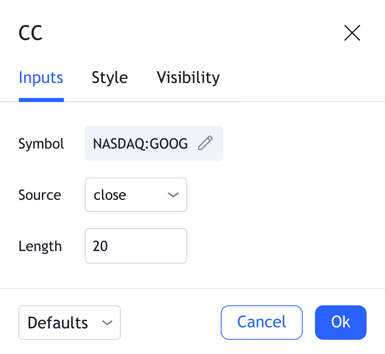
Symbol
The second instrument which will then be compared to the original instrument on the chart.
Length
The time period to be used in calculating the correlation. 20 days is the default.
Source
Determines what data from each bar will be used in calculations. Close is the default.
Style

Correlation
Can toggle the visibility of the Correlation Coefficient as well as the visibility of a price line showing the actual current value of the Correlation Coefficient. Can also select the Correlation Coefficient's color, line thickness and visual style (Area is the Default).
Level
Toggles the visibility and sets price level of three additional horizontal lines. By default, the lines display the maximum and minimum possible values of the correlation coefficient calculation (1 and -1, respectively), as well as the level of zero correlation. It is also possible to set the color, line thickness and select the visual style of each line (the default is Dashed line).