Previous Day High Low Strategy only for LongWelcome to the "Previous Day High Low Strategy only for Long"!.
This strategy aims to identify potential long trading opportunities based on the previous day's high and low prices, along with certain market strength conditions.
Key Features:
Entry Conditions: The strategy triggers a long position when the current day's closing price crosses above the previous day's high or low.
Market Strength Filter: The strategy incorporates a market strength filter using the Average Directional Index (ADX). It only takes long positions when the ADX value is above a specific threshold and when there is a predominance of upward movement.
Trade Timing: The strategy operates within a specified trade window, starting at 09:30 and ending at 15:10. Positions are closed at 15:15 if still active.
Risk Management: The strategy employs dynamic stop-loss and profit-taking levels based on a user-defined Max Profit value. It has three profit targets (T1, T2, T3) and a stop-loss level to manage risk effectively.
Rules:
Ensure that the strategy idea is clearly understandable. Provide an easy-to-read title and a thoughtful description explaining the reasoning behind the strategy.
All content should be ad-free. Avoid any form of promotion, advertising, or solicitation.
No fundraising requests or money solicitation is allowed on TradingView.
Publish in the same language as the TradingView subdomain you're on, except for script titles, which must be in English.
Don't plagiarize. Create and share only unique content, and always give credit when using someone else's work.
Be respectful, kind, and constructive when engaging with others.
Zero tolerance for contentious political discourse, defamatory, threatening, or discriminatory remarks.
Avoid sharing harmful, misleading, or inappropriate content.
Respect the moderators' work and address complaints privately.
Use only your original account and avoid creating duplicate or fake accounts.
Do not attempt to manipulate the reputation system or engage in like-for-like schemes.
Explanation of how the strategy works
1. Previous Day's High and Low (HH, LL):
In this strategy, we start by obtaining the high and low prices of the previous day (not the current day) using the request.security function. This function allows us to access historical data for a specific time frame. The high and low prices are stored in the variables HH and LL, respectively.
2. Entry Conditions:
The strategy uses two conditions to trigger a long position:
Condition 1 (Long Condition 1): If the closing price of the current day crosses above the previous day's high (HH), it generates a long signal. This is achieved using the ta.crossover function, which detects when a crossover occurs.
Condition 2 (Long Condition 2): Similarly, if the closing price of the current day crosses above the previous day's low (LL), it also generates a long signal.
Combined Condition: To take long positions, the strategy combines both long conditions using the logical OR operator (or). This means that if either of the two conditions is met, a long position will be initiated.
3. Market Strength Filter:
The strategy also includes a filter based on the Average Directional Index (ADX) to gauge the market's strength before taking long positions. The ADX measures the strength of a trend in the market. The higher the ADX value, the stronger the trend.
Calculation of ADX: The ADX is calculated using the adx function, which takes two parameters: LWdilength (DMI Length) and LWadxlength (ADX period).
Strength Condition (strength_up): The strategy requires that the ADX value should be above a threshold (11 in this case) and that there is a predominance of upward movement (up > down) before initiating a long position. The LWADX value is multiplied by 2.5 and compared to the highest value of LWADX from the last 4 periods using ta.highest(LWADX , 4). If these conditions are met, the variable strength_up is set to true.
Combined Condition: The strength_up condition is then combined with the long conditions using the logical AND operator (and). This means that the strategy will only take a long position if both the long conditions and the market strength condition are met.
4. Trade Timing:
The strategy sets a specific trade window between 09:30 and 15:10. It will only execute trades within this time frame (TradeTime).
5. Risk Management:
The strategy implements dynamic stop-loss (SL) and profit-taking levels (T1, T2, T3) based on a user-defined Max Profit value. The stop-loss is set as a percentage of the Max Profit value. As the position moves in favor of the trader, the profit targets are adjusted accordingly.
6. Position Management:
The strategy uses the strategy.entry function to enter long positions based on the combined entry conditions. Once a position is open, the script uses strategy.exit to define the exit condition when either the profit target or stop-loss level is hit. The strategy.close function is used to close any open position at the end of the trade window (15:15).
7. Plotting:
The strategy uses the plot function to visualize the previous day's high and low prices, as well as the stop-loss (SL) and profit-taking (T1, T2, T3) levels on the chart.
Overall, the "Previous Day High Low Strategy only for Long" aims to identify potential long trading opportunities based on the previous day's price action and market strength conditions. However, as with any trading strategy, it's essential to thoroughly test it and consider risk management before applying it to real-world trading scenarios.
Disclaimer:
The information presented by this strategy is for educational purposes only and should not be considered as investment advice. The strategy is not designed for qualified investors. Always conduct your own research and consult with a financial advisor before making any trading decisions.
Remember, the success of any trading strategy depends on various factors, including market conditions, risk management, and individual trading skills. Past performance is not indicative of future results.
ค้นหาในสคริปต์สำหรับ "wind+芯片行业+市盈率+财经数据"

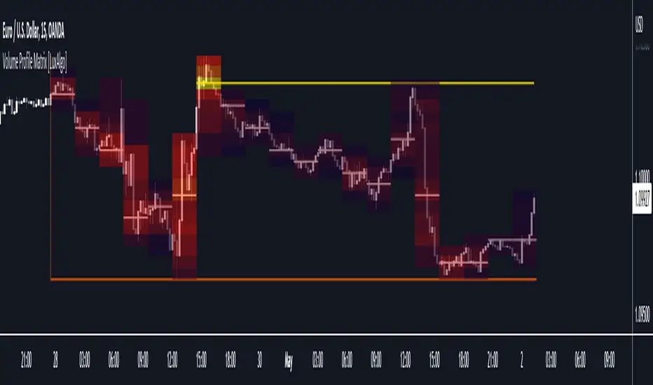
Volume Profile Matrix [LuxAlgo]The Volume Profile Matrix indicator extends from regular volume profiles by also considering calculation intervals within the calculation window rather than only dividing the calculation window in rows.
Note that this indicator is subject to repainting & back-painting, however, treating the indicator as a tool for identifying frequent points of interest can still be very useful.
🔶 SETTINGS
Lookback: Number of most recent bars used to calculate the indicator.
Columns: Number of columns (intervals) used to calculate the volume profile matrix.
Rows: Number of rows (intervals) used to calculate the volume profile matrix.
🔶 USAGE
The Volume Profile Matrix indicator can be used to obtain more information regarding liquidity on specific time intervals. Instead of simply dividing the calculation window into equidistant rows, the calculation is done through a grid.
Grid cells with trading activity occurring inside them are colored. More activity is highlighted through a gradient and by default, cells with a color that are closer to red indicate that more trading activity took place within that cell. The cell with the highest amount of trading activity is always highlighted in yellow.
Each interval (column) includes a point of control which highlights an estimate of the price level with the highest traded volume on that interval. The level with the highest traded volume of the overall grid is extended to the most recent bar.
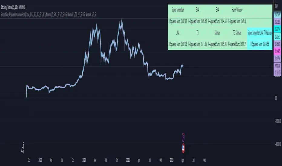
Smoothing R-Squared ComparisonIntroduction
Heyo guys, here I made a comparison between my favorised smoothing algorithms.
I chose the R-Squared value as rating factor to accomplish the comparison.
The indicator is non-repainting.
Description
In technical analysis, traders often use moving averages to smooth out the noise in price data and identify trends. While moving averages are a useful tool, they can also obscure important information about the underlying relationship between the price and the smoothed price.
One way to evaluate this relationship is by calculating the R-squared value, which represents the proportion of the variance in the price that can be explained by the smoothed price in a linear regression model.
This PineScript code implements a smoothing R-squared comparison indicator.
It provides a comparison of different smoothing techniques such as Kalman filter, T3, JMA, EMA, SMA, Super Smoother and some special combinations of them.
The Kalman filter is a mathematical algorithm that uses a series of measurements observed over time, containing statistical noise and other inaccuracies, and produces estimates of unknown variables that tend to be more accurate than those based on a single measurement.
The input parameters for the Kalman filter include the process noise covariance and the measurement noise covariance, which help to adjust the sensitivity of the filter to changes in the input data.
The T3 smoothing technique is a popular method used in technical analysis to remove noise from a signal.
The input parameters for the T3 smoothing method include the length of the window used for smoothing, the type of smoothing used (Normal or New), and the smoothing factor used to adjust the sensitivity to changes in the input data.
The JMA smoothing technique is another popular method used in technical analysis to remove noise from a signal.
The input parameters for the JMA smoothing method include the length of the window used for smoothing, the phase used to shift the input data before applying the smoothing algorithm, and the power used to adjust the sensitivity of the JMA to changes in the input data.
The EMA and SMA techniques are also popular methods used in technical analysis to remove noise from a signal.
The input parameters for the EMA and SMA techniques include the length of the window used for smoothing.
The indicator displays a comparison of the R-squared values for each smoothing technique, which provides an indication of how well the technique is fitting the data.
Higher R-squared values indicate a better fit. By adjusting the input parameters for each smoothing technique, the user can compare the effectiveness of different techniques in removing noise from the input data.
Usage
You can use it to find the best fitting smoothing method for the timeframe you usually use.
Just apply it on your preferred timeframe and look for the highlighted table cell.
Conclusion
It seems like the T3 works best on timeframes under 4H.
There's where I am active, so I will use this one more in the future.
Thank you for checking this out. Enjoy your day and leave me a like or comment. 🧙♂️
---
Credits to:
▪@loxx – T3
▪@balipour – Super Smoother
▪ChatGPT – Wrote 80 % of this article and helped with the research
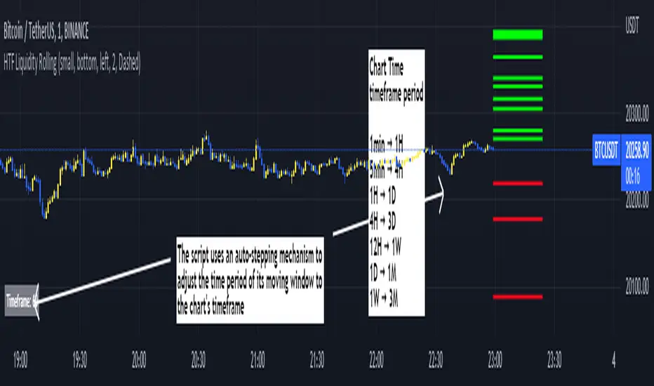
Rolling HTF Liquidity Levels [CHE]█ OVERVIEW
This indicator displays a Rolling HTF Liquidity Levels . Contrary to HTF Liquidity Levels indicators which use a fix time segment, Rolling HTF Liquidity Levels calculates using a moving window defined by a time period (not a simple number of bars), so it shows better results.
This indicator is inspired by
The indicator introduces a new representation of the previous rolling time frame highs & lows (DWM HL) with a focus on untapped levels.
█ CONCEPTS
Untapped Levels
It is popularly known that the liquidity is located behind swing points or beyond higher time frames highs/lows.
Rolling HTF Liquidity Levels uses a moving window, it does not exhibit the static of the HTF Liquidity Levels plots.
█ HOW TO USE IT
Load the indicator on an active chart (see the Help Center if you don't know how).
Time period
By default, the script uses an auto-stepping mechanism to adjust the time period of its moving window to the chart's timeframe. The following table shows chart timeframes and the corresponding time period used by the script. When the chart's timeframe is less than or equal to the timeframe in the first column, the second column's time period is used to calculate the Rolling HTF Liquidity Levels:
Chart Time
timeframe period
1min 🠆 1H
5min 🠆 4H
1H 🠆 1D
4H 🠆 3D
12H 🠆 1W
1D 🠆 1M
1W 🠆 3M
By default, the time period currently used is displayed in the lower-right corner of the chart. The script's inputs allow you to hide the display or change its size and location.
This indicator should make trading easier and improve analysis. Nothing is worse than indicators that give confusingly different signals.
I hope you enjoy my new ideas
best regards
Chervolino
z_score_bgd
Z-score indicator for volatile currency pairs, showing STRONG BUY, BUY, SELL, STRONG SELL zones by shading the chart background.
---------------------------------
Background
---------------------------------
Based on mean reversion, a theory that after a swing in price the price will tend back to the mean. This offers some ability to predict future trends.
The formula for calculating a z-score is is z = (x-μ)/σ, where x is the pair price, μ is the mean for a population, and σ is the population standard deviation.
---------------------------------
Set up
---------------------------------
The user can define their own value for the "window" or population, which is the number of preceding days to evaluate. This value will affect the frequency and magnitude of trades, with higher "window" values reducing the frequency of reversions but increasing their magnitude.
Where the value for "window" is left at 99, the default values below will be applied in the background. Otherwise the user's selection will be in effect.
atombtc 18
avaxbtc 21
ethbtc 18
ftmbtc 11
maticbtc 11
solbtc 11
soleth 16
The default values above are intended for the daily time-frame.
---------------------------------
Interpreting the indicator
---------------------------------
Dark green -> large deviation below mean price (strong buy)
Green -> moderate deviation below mean price (buy)
Red -> moderate deviation below mean price (sell)
Dark red -> large deviation below mean price (strong sell)
Z-score is an imperfect indicator, as with all indiciators and trading decisions must be confirmed by multiple indicators and consider other factors.

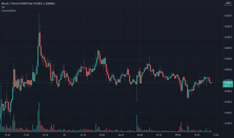
CommonFiltersLibrary "CommonFilters"
Collection of some common Filters and Moving Averages. This collection is not encyclopaedic, but to declutter my other scripts. Suggestions are welcome, though. Many filters here are based on the work of John F. Ehlers
sma(src, len) Simple Moving Average
Parameters:
src : Series to use
len : Filtering length
Returns: Filtered series
ema(src, len) Exponential Moving Average
Parameters:
src : Series to use
len : Filtering length
Returns: Filtered series
rma(src, len) Wilder's Smoothing (Running Moving Average)
Parameters:
src : Series to use
len : Filtering length
Returns: Filtered series
hma(src, len) Hull Moving Average
Parameters:
src : Series to use
len : Filtering length
Returns: Filtered series
vwma(src, len) Volume Weighted Moving Average
Parameters:
src : Series to use
len : Filtering length
Returns: Filtered series
hp2(src) Simple denoiser
Parameters:
src : Series to use
Returns: Filtered series
fir2(src) Zero at 2 bar cycle period by John F. Ehlers
Parameters:
src : Series to use
Returns: Filtered series
fir3(src) Zero at 3 bar cycle period by John F. Ehlers
Parameters:
src : Series to use
Returns: Filtered series
fir23(src) Zero at 2 bar and 3 bar cycle periods by John F. Ehlers
Parameters:
src : Series to use
Returns: Filtered series
fir234(src) Zero at 2, 3 and 4 bar cycle periods by John F. Ehlers
Parameters:
src : Series to use
Returns: Filtered series
hp(src, len) High Pass Filter for cyclic components shorter than langth. Part of Roofing Filter by John F. Ehlers
Parameters:
src : Series to use
len : Filtering length
Returns: Filtered series
supers2(src, len) 2-pole Super Smoother by John F. Ehlers
Parameters:
src : Series to use
len : Filtering length
Returns: Filtered series
filt11(src, len) Filt11 is a variant of 2-pole Super Smoother with error averaging for zero-lag response by John F. Ehlers
Parameters:
src : Series to use
len : Filtering length
Returns: Filtered series
supers3(src, len) 3-pole Super Smoother by John F. Ehlers
Parameters:
src : Series to use
len : Filtering length
Returns: Filtered series
hannFIR(src, len) Hann Window Filter by John F. Ehlers
Parameters:
src : Series to use
len : Filtering length
Returns: Filtered series
hammingFIR(src, len) Hamming Window Filter (inspired by John F. Ehlers). Simplified implementation as Pedestal input parameter cannot be supplied, so I calculate it from the supplied length
Parameters:
src : Series to use
len : Filtering length
Returns: Filtered series
triangleFIR(src, len) Triangle Window Filter by John F. Ehlers
Parameters:
src : Series to use
len : Filtering length
Returns: Filtered series
doPrefilter(type, src) Execute a particular Prefilter from the list
Parameters:
type : Prefilter type to use
src : Series to use
Returns: Filtered series
doMA(type, src, len) Execute a particular MA from the list
Parameters:
type : MA type to use
src : Series to use
len : Filtering length
Returns: Filtered series
VPA - 5.0 This is a upgraded version of the vpa analysis script which basically implements Volume Spread Analysis (aka Volume Price analysis). It has been rechristened as VPA 5.0 to be inline with version released for Amiboker package so that all future upgrades will go hand in hand. All most all featured of the Amibroker version has been incorporated in this version. Some important additions are as follows
1. A status window for the bar and Trend Description added. No need to plot the trend bands or additional trend Indicator any more.
2. The most important upgrade would be the addition of a Alert window which provides description of the VSA signals. It is also a log window which provides up to 10 last signals
(Credits to Quantnomad for this wonderful piece of code. This feature is an adaptation of his public code)
3. Added facility to plot EMAs / PEMAs with changable parameters
4. Added facility to plot VWAP
5. Facility to switch on and Off the VSA signals. Also tool tip provides description of the signals
6. Facility to plot Resistance and Volume Lines (Credits to @margepadu)
Hope this script will be helpful to everyone. Please do provide your feedback and suggestions for improvements

Fast Fourier Transform (FFT) FilterDear friends!
I'm happy to present an implementation of the Fast Fourier Transform (FFT) algorithm. The script uses the FFT procedure to decompose the input time series into its cyclical constituents, in other words, its frequency components , and convert it back to the time domain with modified frequency content, that is, to filter it.
Input Description and Usage
Source and Length :
Indicates where the data comes from and the size of the lookback window used to build the dataset.
Standardize Input Dataset :
If enabled, the dataset is preprocessed by subtracting its mean and normalizing the result by the standard deviation, which is sometimes useful when analyzing seasonalities. This procedure is not recommended when using the FFT filter for smoothing (see below), as it will not preserve the average of the dataset.
Show Frequency-Domain Power Spectrum :
When enabled, the results of Fourier analysis (for the last price bar!) are plotted as a frequency-domain power spectrum , where “power” is a measure of the significance of the component in the dataset. In the spectrum, lower frequencies (longer cycles) are on the right, higher frequencies are on the left. The graph does not display the 0th component, which contains only information about the mean value. Frequency components that are allowed to pass through the filter (see below) are highlighted in magenta .
Dominant Cycles, Rows :
If this option is activated, the periods and relative powers of several dominant cyclical components that is, those that have a higher power, are listed in the table. The number of the component in the power spectrum (N) is shown in the first column. The number of rows in the table is defined by the user.
Show Inverse Fourier Transform (Filtered) :
When enabled, the reconstructed and filtered time-domain dataset (for the last price bar!) is displayed.
Apply FFT Filter in a Moving Window :
When enabled, the FFT filter with the same parameters is applied to each bar. The last data point of the reconstructed and filtered dataset is used to build a new time series. For example, by getting rid of high-frequency noise, the FFT filter can make the data smoother. By removing slowly evolving low-frequency components (including non-periodic constituents), one can reveal and analyze shorter cycles. Since filtering is done in real-time in a moving window (similar to the moving average), the modified data can potentially be used as part of a strategy and be subjected to other technical indicators.
Lowest Allowed N :
Indicates the number of the lowest frequency component used in the reconstructed time series.
Highest Allowed N :
Indicates the number of the highest frequency component used in the reconstructed time series.
Filtering Time Range block:
Specifies the time range over which real-time FFT filtering is applied. The reason for the presence of this block is that the FFT procedure is relatively computationally intensive. Therefore, the script execution may encounter the time limit imposed by TradingView when all historical bars are processed.
As always, I look forward to your feedback!
Also, leave a comment if you'd be interested in the tutorial on how to use this tool and/or in seeing the FFT filter in a strategy.

[blackcat] L2 Ehlers Center of GravityLevel: 2
Background
John F. Ehlers introuced center of gravity (CG) in his "Cybernetic Analysis for Stocks and Futures" chapter 5 on 2004.
Function
The center of gravity (CG) of a physical object is its balance point. For example, if you balance a 12-inch ruler on your finger, the CG will be at its 6-inch point. If you change the weight distribution of the ruler by putting a paper clip on one end, then the balance point (i.e., the CG) shifts toward
the paper clip. Moving from the physical world to the trading world, we can substitute the prices over our window of observation for the units of weight along the ruler. Using this analogy, we see that the CG of the window moves to the right when prices increase sharply. Correspondingly, the CG of the window moves to the left when prices decrease.
The idea of computing the center of gravity of Dr. Ehlers arose from observing how the lags of various finite impulse response (FIR) filters vary according to
the relative amplitude of the filter coefficients. A simple moving average (SMA) is an FIR filter where all the filter coefficients have the same value (usually unity). As a result, the CG of the SMA is exactly in the center of the filter. A weighted moving average (WMA) is an FIR filter where the most recent price is weighted by the length of the filter, the next most recent price is weighted by the length of the filter less 1, and so on. The weighting terms are the filter coefficients. The filter coefficients of a WMA describe the outline of a triangle. It is well known that the CG of a triangle is located at one-third the length of the base of the triangle. In other words, the CG of the WMA has shifted to the right relative to the CG of an SMA of equal length, resulting in less lag. In all FIR filters, the sum of the product of the coefficients and prices must be divided by the sum of the coefficients so that the scale of the original prices is retained.
Key Signal
CG ---> CG fast line
CG (2) ---> CG slow line
Pros and Cons
100% John F. Ehlers definition translation of original work, even variable names are the same. This help readers who would like to use pine to read his book. If you had read his works, then you will be quite familiar with my code style.
Remarks
The 26th script for Blackcat1402 John F. Ehlers Week publication.
Readme
In real life, I am a prolific inventor. I have successfully applied for more than 60 international and regional patents in the past 12 years. But in the past two years or so, I have tried to transfer my creativity to the development of trading strategies. Tradingview is the ideal platform for me. I am selecting and contributing some of the hundreds of scripts to publish in Tradingview community. Welcome everyone to interact with me to discuss these interesting pine scripts.
The scripts posted are categorized into 5 levels according to my efforts or manhours put into these works.
Level 1 : interesting script snippets or distinctive improvement from classic indicators or strategy. Level 1 scripts can usually appear in more complex indicators as a function module or element.
Level 2 : composite indicator/strategy. By selecting or combining several independent or dependent functions or sub indicators in proper way, the composite script exhibits a resonance phenomenon which can filter out noise or fake trading signal to enhance trading confidence level.
Level 3 : comprehensive indicator/strategy. They are simple trading systems based on my strategies. They are commonly containing several or all of entry signal, close signal, stop loss, take profit, re-entry, risk management, and position sizing techniques. Even some interesting fundamental and mass psychological aspects are incorporated.
Level 4 : script snippets or functions that do not disclose source code. Interesting element that can reveal market laws and work as raw material for indicators and strategies. If you find Level 1~2 scripts are helpful, Level 4 is a private version that took me far more efforts to develop.
Level 5 : indicator/strategy that do not disclose source code. private version of Level 3 script with my accumulated script processing skills or a large number of custom functions. I had a private function library built in past two years. Level 5 scripts use many of them to achieve private trading strategy.

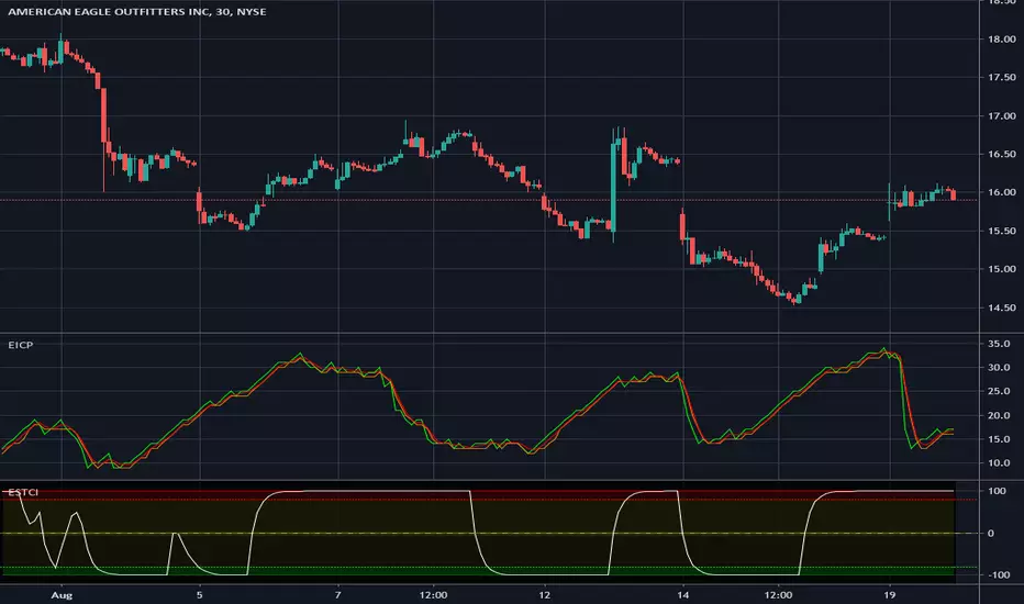
Enhanced Instantaneous Cycle Period - Dr. John EhlersThis is my first public release of detector code entitled "Enhanced Instantaneous Cycle Period" for PSv4.0 I built many months ago. Be forewarned, this is not an indicator, this is a detector to be used by ADVANCED developers to build futuristic indicators in Pine. The origins of this script come from a document by Dr. John Ehlers entitled "SIGNAL ANALYSIS CONCEPTS". You may find this using the NSA's reverse search engine "goggles", as I call it. John Ehlers' MESA used this measurement to establish the data window for analysis for MESA Cycle computations. So... does any developer wish to emulate MESA Cycle now??
I decided to take instantaneous cycle period to another level of novel attainability in this public release of source code with the following methods, if you are curious how I ENHANCED it. Firstly I reduced the delay of accurate measurement from bar_index==0 by quite a few bars closer to IPO. Secondarily, I provided a limit of 6 for a minimum instantaneous cycle period. At bar_index==0, it would provide a period of 0 wrecking many algorithms from the start. I also increased the instantaneous cycle period's maximum value to 80 from 50, providing a window of 6-80 for the instantaneous cycle period value window limits. Thirdly, I replaced the internal EMA with another algorithm. It reduces the lag while extracting a floating point number, for algorithms that will accept that, compared to a sluggish ordinary EMA return. You will see the excessive EMA delay with adding plot(ema(ICP,7)) as it was originally designed. Lastly it's in one simple function for reusability in a nice little package comprising of less than 40 lines of code. I hope I explained that adequately enough and gave you the reader a glimpse of the "Power of Pine" combined with ingenuity.
Be forewarned again, that most of Pine's built-in functions will not accept a floating-point number or dynamic integers for the "length" of it's calculation. You will have to emulate the built-in functions by creating Pine based custom functions, and I assure you, this is very possible in many cases, but not all without array support. You may use int(ICP) to extract an integer from the smoothICP return variable, which may be favorable compared to the choppiness/ringing if ICP alone.
This is commonly what my dense intricate code looks like behind the veil. If you are wondering why there is barely any notation, that's because the notation is in the variable naming and this is intended primarily for ADVANCED developers too. It does contain lines of code that explore techniques in Pine that may be applicable in other Pine projects for those learning or wishing to excel with Pine.
Showcased in the chart below is my free to use "Enhanced Schaff Trend Cycle Indicator", having a common appeal to TV users frequently. If you do have any questions or comments regarding this indicator, I will consider your inquiries, thoughts, and ideas presented below in the comments section, when time provides it. As always, "Like" it if you simply just like it with a proper thumbs up, and also return to my scripts list occasionally for additional postings. Have a profitable future everyone!
NOTICE: Copy pasting bandits who may be having nefarious thoughts, DO NOT attempt this, because this may violate Tradingview's terms, conditions and/or house rules. "WE" are always watching the TV community vigilantly for mischievous behaviors and actions that exploit well intended authors for the purpose of increasing brownie points in reputation scores. Hiding behind a "protected" wall may not protect you from investigation and account penalization by TV staff. Be respectful, and don't just throw an ma() in there branding it as "your" gizmo. Fair enough? Alrighty then... I firmly believe in "innovating" future state-of-the-art indicators, and please contact me if you wish to do so.
Globex Trap w/ percentage [SLICKRICK]Globex Trap w/ Percentage
Overview
The Globex Trap w/ Percentage indicator is a powerful tool designed to help traders identify high-probability trading opportunities by analyzing price action during the Globex (overnight) session and regular trading hours. By combining Globex session ranges with Supply & Demand zones, this indicator highlights potential "trap" areas where significant price reactions may occur. Additionally, it calculates the Globex session range as a percentage of the daily Average True Range (ATR), providing valuable context for assessing market volatility.
This indicator is ideal for traders in futures markets or other instruments traded during Globex sessions, offering a visual and analytical edge for spotting key price levels and potential reversals or breakouts.
Key Features
Globex Session Tracking:
Visualizes the high and low of the Globex session (default: 3:00 PM to 6:30 AM PST) with customizable time settings.
Displays a semi-transparent box to mark the Globex range, with labels for "Globex High" and "Globex Low."
Calculates the Globex range as a percentage of the daily ATR, displayed as a label for quick reference.
Supply & Demand Zones:
Identifies Supply & Demand zones during regular trading hours (default: 6:00 AM to 8:00 AM PST) with customizable time settings.
Draws semi-transparent boxes to highlight these zones, aiding in the identification of key support and resistance areas.
Trap Area Identification:
Highlights potential trap zones where Globex ranges and Supply & Demand zones overlap, indicating areas where price may reverse or consolidate due to trapped traders.
Customizable Settings:
Adjust Globex and Supply & Demand session times to suit your trading preferences.
Toggle visibility of Globex and Supply & Demand zones independently.
Customize box colors for better chart readability.
Set the lookback period (default: 10 days) to control how many historical zones are displayed.
Configure the ATR length (default: 14) for the percentage calculation.
PST Timezone Default:
All times are based on Pacific Standard Time (PST) by default, ensuring accurate session tracking for users in this timezone or those aligning with U.S. West Coast market hours.
Recommended Usage
Timeframes: Best used on 1-hour charts or lower (e.g., 15-minute, 5-minute) for precise entry and exit points.
Markets: Optimized for futures (e.g., ES, NQ, CL) and other instruments traded during Globex sessions.
Historical Data: Ensure at least 10 days of historical data for optimal visualization of zones.
Strategy Integration: Use the indicator to identify potential reversals or breakouts at Globex highs/lows or Supply & Demand zones. The ATR percentage provides context for whether the Globex range is significant relative to typical daily volatility.
How It Works
Globex Session:
Tracks the high and low prices during the user-defined Globex session (default: 3:00 PM to 6:30 AM PST).
When the session ends, a box is drawn from the start to the end of the session, capturing the high and low prices.
Labels are placed at the midpoint of the session, showing "Globex High," "Globex Low," and the range as a percentage of the daily ATR (e.g., "75.23% of Daily ATR").
Supply & Demand Zones:
Tracks the high and low prices during the user-defined regular trading hours (default: 6:00 AM to 8:00 AM PST).
Draws a box to mark these zones, which often act as key support or resistance levels.
ATR Percentage:
Calculates the Globex range (high minus low) and divides it by the daily ATR to express it as a percentage.
This metric helps traders gauge whether the overnight price movement is significant compared to the instrument’s typical volatility.
Time Handling:
Uses PST (UTC-8) for all time calculations, ensuring accurate session timing for users aligning with this timezone.
Properly handles overnight sessions that cross midnight, ensuring seamless tracking.
Input Settings
Globex Session Settings:
Show Globex Session: Enable/disable Globex session visualization (default: true).
Globex Start/End Time: Set the start and end times for the Globex session (default: 3:00 PM to 6:30 AM PST).
Globex Box Color: Customize the color of the Globex session box (default: semi-transparent gray).
Supply & Demand Zone Settings:
Show Supply & Demand Zone: Enable/disable zone visualization (default: true).
Zone Start/End Time: Set the start and end times for Supply & Demand zones (default: 6:00 AM to 8:00 AM PST).
Zone Box Color: Customize the color of the zone box (default: semi-transparent aqua).
General Settings:
Days to Look Back: Number of historical days to display zones (default: 10).
ATR Length: Period for calculating the daily ATR (default: 14).
Notes
All times are in Pacific Standard Time (PST). Adjust the start and end times if your market operates in a different timezone or if you prefer different session windows.
The indicator is optimized for instruments with active Globex sessions, such as futures. Results may vary for non-24/5 markets.
A typo in the label "Globe Low" (should be "Globex Low") will be corrected in future updates.
Ensure your TradingView chart is set to display sufficient historical data to view the full lookback period.
Why Use This Indicator?
The Globex Trap w/ Percentage indicator provides a unique combination of session-based range analysis, Supply & Demand zone identification, and volatility context via the ATR percentage. Whether you’re a day trader, swing trader, or scalper, this tool helps you:
Pinpoint key price levels where institutional traders may act.
Assess the significance of overnight price movements relative to daily volatility.
Identify potential trap zones for high-probability setups.
Customize the indicator to fit your trading style and market preferences.

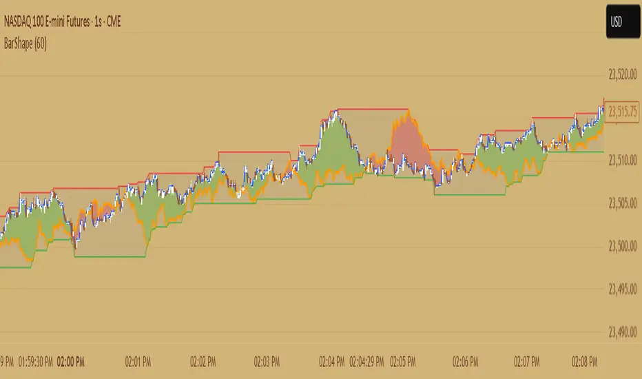
Candle ShapeCandle Shape
This indicator visualizes rolling candles that aggregate price action over a chosen lookback period, allowing you to see how OHLC dynamics evolve in real time.
Instead of waiting for a higher timeframe (HTF) bar to close, you can track its development directly from a lower timeframe chart.
For example, view how a 1-hour candle is forming on a 1-minute chart — complete with rolling open, high, low, and close levels, as well as colored body and wick areas.
---
🔹 How it works
- Lookback Period (n) → sets the bucket size, defining how many bars are merged into a “meta-candle.”
- The script continuously updates the meta-open, meta-high, meta-low, and meta-close.
- Body and wick areas are filled with color , making bullish/bearish transitions easy to follow.
---
🔹 Use cases
- Monitor the intra-development of higher timeframe candles.
- Analyze rolling OHLC structures to understand how price dynamics shift across different aggregation windows.
- Explore unique perspectives for strategy confirmation, breakout anticipation, and market structure analysis.
---
✨ Candle Shape bridges the gap between timeframes and uncovers new layers of price interaction.
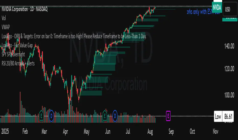
RSI 20/80 Arrows + AlertsRSI 20/80 Arrows + Alerts
This indicator is a modified Relative Strength Index (RSI) tool designed to help traders spot potential overbought and oversold conditions using customizable threshold levels (default 80 for overbought, 20 for oversold).
Features:
Custom RSI Levels – Default to 80/20 instead of the standard 70/30, but fully adjustable by the user.
Visual Signals –
Blue Arrow Up appears below the bar when RSI crosses up from below the oversold level (potential buy zone).
Red Arrow Down appears above the bar when RSI crosses down from above the overbought level (potential sell zone).
Alerts Built In – Receive notifications when either signal occurs, with the option to confirm signals only on bar close for reduced noise.
Guide Levels – Optionally display overbought/oversold reference lines on the chart for quick visual reference.
Overlay Mode – Signals are plotted directly on the price chart, so you don’t need to switch between chart windows.
Use Case:
Ideal for traders who want quick, visual confirmation of potential turning points based on RSI, especially in strategies where more extreme levels (like 20/80) help filter out weaker signals. Works well across all markets and timeframes.
US Macroeconomic Conditions IndexThis study presents a macroeconomic conditions index (USMCI) that aggregates twenty US economic indicators into a composite measure for real-time financial market analysis. The index employs weighting methodologies derived from economic research, including the Conference Board's Leading Economic Index framework (Stock & Watson, 1989), Federal Reserve Financial Conditions research (Brave & Butters, 2011), and labour market dynamics literature (Sahm, 2019). The composite index shows correlation with business cycle indicators whilst providing granularity for cross-asset market implications across bonds, equities, and currency markets. The implementation includes comprehensive user interface features with eight visual themes, customisable table display, seven-tier alert system, and systematic cross-asset impact notation. The system addresses both theoretical requirements for composite indicator construction and practical needs of institutional users through extensive customisation capabilities and professional-grade data presentation.
Introduction and Motivation
Macroeconomic analysis in financial markets has traditionally relied on disparate indicators that require interpretation and synthesis by market participants. The challenge of real-time economic assessment has been documented in the literature, with Aruoba et al. (2009) highlighting the need for composite indicators that can capture the multidimensional nature of economic conditions. Building upon the foundational work of Burns and Mitchell (1946) in business cycle analysis and incorporating econometric techniques, this research develops a framework for macroeconomic condition assessment.
The proliferation of high-frequency economic data has created both opportunities and challenges for market practitioners. Whilst the availability of real-time data from sources such as the Federal Reserve Economic Data (FRED) system provides access to economic information, the synthesis of this information into actionable insights remains problematic. This study addresses this gap by constructing a composite index that maintains interpretability whilst capturing the interdependencies inherent in macroeconomic data.
Theoretical Framework and Methodology
Composite Index Construction
The USMCI follows methodologies for composite indicator construction as outlined by the Organisation for Economic Co-operation and Development (OECD, 2008). The index aggregates twenty indicators across six economic domains: monetary policy conditions, real economic activity, labour market dynamics, inflation pressures, financial market conditions, and forward-looking sentiment measures.
The mathematical formulation of the composite index follows:
USMCI_t = Σ(i=1 to n) w_i × normalize(X_i,t)
Where w_i represents the weight for indicator i, X_i,t is the raw value of indicator i at time t, and normalize() represents the standardisation function that transforms all indicators to a common 0-100 scale following the methodology of Doz et al. (2011).
Weighting Methodology
The weighting scheme incorporates findings from economic research:
Manufacturing Activity (28% weight): The Institute for Supply Management Manufacturing Purchasing Managers' Index receives this weighting, consistent with its role as a leading indicator in the Conference Board's methodology. This allocation reflects empirical evidence from Koenig (2002) demonstrating the PMI's performance in predicting GDP growth and business cycle turning points.
Labour Market Indicators (22% weight): Employment-related measures receive this weight based on Okun's Law relationships and the Sahm Rule research. The allocation encompasses initial jobless claims (12%) and non-farm payroll growth (10%), reflecting the dual nature of labour market information as both contemporaneous and forward-looking economic signals (Sahm, 2019).
Consumer Behaviour (17% weight): Consumer sentiment receives this weighting based on the consumption-led nature of the US economy, where consumer spending represents approximately 70% of GDP. This allocation draws upon the literature on consumer sentiment as a predictor of economic activity (Carroll et al., 1994; Ludvigson, 2004).
Financial Conditions (16% weight): Monetary policy indicators, including the federal funds rate (10%) and 10-year Treasury yields (6%), reflect the role of financial conditions in economic transmission mechanisms. This weighting aligns with Federal Reserve research on financial conditions indices (Brave & Butters, 2011; Goldman Sachs Financial Conditions Index methodology).
Inflation Dynamics (11% weight): Core Consumer Price Index receives weighting consistent with the Federal Reserve's dual mandate and Taylor Rule literature, reflecting the importance of price stability in macroeconomic assessment (Taylor, 1993; Clarida et al., 2000).
Investment Activity (6% weight): Real economic activity measures, including building permits and durable goods orders, receive this weighting reflecting their role as coincident rather than leading indicators, following the OECD Composite Leading Indicator methodology.
Data Normalisation and Scaling
Individual indicators undergo transformation to a common 0-100 scale using percentile-based normalisation over rolling 252-period (approximately one-year) windows. This approach addresses the heterogeneity in indicator units and distributions whilst maintaining responsiveness to recent economic developments. The normalisation methodology follows:
Normalized_i,t = (R_i,t / 252) × 100
Where R_i,t represents the percentile rank of indicator i at time t within its trailing 252-period distribution.
Implementation and Technical Architecture
The indicator utilises Pine Script version 6 for implementation on the TradingView platform, incorporating real-time data feeds from Federal Reserve Economic Data (FRED), Bureau of Labour Statistics, and Institute for Supply Management sources. The architecture employs request.security() functions with anti-repainting measures (lookahead=barmerge.lookahead_off) to ensure temporal consistency in signal generation.
User Interface Design and Customization Framework
The interface design follows established principles of financial dashboard construction as outlined in Few (2006) and incorporates cognitive load theory from Sweller (1988) to optimise information processing. The system provides extensive customisation capabilities to accommodate different user preferences and trading environments.
Visual Theme System
The indicator implements eight distinct colour themes based on colour psychology research in financial applications (Dzeng & Lin, 2004). Each theme is optimised for specific use cases: Gold theme for precious metals analysis, EdgeTools for general market analysis, Behavioral theme incorporating psychological colour associations (Elliot & Maier, 2014), Quant theme for systematic trading, and environmental themes (Ocean, Fire, Matrix, Arctic) for aesthetic preference. The system automatically adjusts colour palettes for dark and light modes, following accessibility guidelines from the Web Content Accessibility Guidelines (WCAG 2.1) to ensure readability across different viewing conditions.
Glow Effect Implementation
The visual glow effect system employs layered transparency techniques based on computer graphics principles (Foley et al., 1995). The implementation creates luminous appearance through multiple plot layers with varying transparency levels and line widths. Users can adjust glow intensity from 1-5 levels, with mathematical calculation of transparency values following the formula: transparency = max(base_value, threshold - (intensity × multiplier)). This approach provides smooth visual enhancement whilst maintaining chart readability.
Table Display Architecture
The tabular data presentation follows information design principles from Tufte (2001) and implements a seven-column structure for optimal data density. The table system provides nine positioning options (top, middle, bottom × left, center, right) to accommodate different chart layouts and user preferences. Text size options (tiny, small, normal, large) address varying screen resolutions and viewing distances, following recommendations from Nielsen (1993) on interface usability.
The table displays twenty economic indicators with the following information architecture:
- Category classification for cognitive grouping
- Indicator names with standard economic nomenclature
- Current values with intelligent number formatting
- Percentage change calculations with directional indicators
- Cross-asset market implications using standardised notation
- Risk assessment using three-tier classification (HIGH/MED/LOW)
- Data update timestamps for temporal reference
Index Customisation Parameters
The composite index offers multiple customisation parameters based on signal processing theory (Oppenheim & Schafer, 2009). Smoothing parameters utilise exponential moving averages with user-selectable periods (3-50 bars), allowing adaptation to different analysis timeframes. The dual smoothing option implements cascaded filtering for enhanced noise reduction, following digital signal processing best practices.
Regime sensitivity adjustment (0.1-2.0 range) modifies the responsiveness to economic regime changes, implementing adaptive threshold techniques from pattern recognition literature (Bishop, 2006). Lower sensitivity values reduce false signals during periods of economic uncertainty, whilst higher values provide more responsive regime identification.
Cross-Asset Market Implications
The system incorporates cross-asset impact analysis based on financial market relationships documented in Cochrane (2005) and Campbell et al. (1997). Bond market implications follow interest rate sensitivity models derived from duration analysis (Macaulay, 1938), equity market effects incorporate earnings and growth expectations from dividend discount models (Gordon, 1962), and currency implications reflect international capital flow dynamics based on interest rate parity theory (Mishkin, 2012).
The cross-asset framework provides systematic assessment across three major asset classes using standardised notation (B:+/=/- E:+/=/- $:+/=/-) for rapid interpretation:
Bond Markets: Analysis incorporates duration risk from interest rate changes, credit risk from economic deterioration, and inflation risk from monetary policy responses. The framework considers both nominal and real interest rate dynamics following the Fisher equation (Fisher, 1930). Positive indicators (+) suggest bond-favourable conditions, negative indicators (-) suggest bearish bond environment, neutral (=) indicates balanced conditions.
Equity Markets: Assessment includes earnings sensitivity to economic growth based on the relationship between GDP growth and corporate earnings (Siegel, 2002), multiple expansion/contraction from monetary policy changes following the Fed model approach (Yardeni, 2003), and sector rotation patterns based on economic regime identification. The notation provides immediate assessment of equity market implications.
Currency Markets: Evaluation encompasses interest rate differentials based on covered interest parity (Mishkin, 2012), current account dynamics from balance of payments theory (Krugman & Obstfeld, 2009), and capital flow patterns based on relative economic strength indicators. Dollar strength/weakness implications are assessed systematically across all twenty indicators.
Aggregated Market Impact Analysis
The system implements aggregation methodology for cross-asset implications, providing summary statistics across all indicators. The aggregated view displays count-based analysis (e.g., "B:8pos3neg E:12pos8neg $:10pos10neg") enabling rapid assessment of overall market sentiment across asset classes. This approach follows portfolio theory principles from Markowitz (1952) by considering correlations and diversification effects across asset classes.
Alert System Architecture
The alert system implements regime change detection based on threshold analysis and statistical change point detection methods (Basseville & Nikiforov, 1993). Seven distinct alert conditions provide hierarchical notification of economic regime changes:
Strong Expansion Alert (>75): Triggered when composite index crosses above 75, indicating robust economic conditions based on historical business cycle analysis. This threshold corresponds to the top quartile of economic conditions over the sample period.
Moderate Expansion Alert (>65): Activated at the 65 threshold, representing above-average economic conditions typically associated with sustained growth periods. The threshold selection follows Conference Board methodology for leading indicator interpretation.
Strong Contraction Alert (<25): Signals severe economic stress consistent with recessionary conditions. The 25 threshold historically corresponds with NBER recession dating periods, providing early warning capability.
Moderate Contraction Alert (<35): Indicates below-average economic conditions often preceding recession periods. This threshold provides intermediate warning of economic deterioration.
Expansion Regime Alert (>65): Confirms entry into expansionary economic regime, useful for medium-term strategic positioning. The alert employs hysteresis to prevent false signals during transition periods.
Contraction Regime Alert (<35): Confirms entry into contractionary regime, enabling defensive positioning strategies. Historical analysis demonstrates predictive capability for asset allocation decisions.
Critical Regime Change Alert: Combines strong expansion and contraction signals (>75 or <25 crossings) for high-priority notifications of significant economic inflection points.
Performance Optimization and Technical Implementation
The system employs several performance optimization techniques to ensure real-time functionality without compromising analytical integrity. Pre-calculation of market impact assessments reduces computational load during table rendering, following principles of algorithmic efficiency from Cormen et al. (2009). Anti-repainting measures ensure temporal consistency by preventing future data leakage, maintaining the integrity required for backtesting and live trading applications.
Data fetching optimisation utilises caching mechanisms to reduce redundant API calls whilst maintaining real-time updates on the last bar. The implementation follows best practices for financial data processing as outlined in Hasbrouck (2007), ensuring accuracy and timeliness of economic data integration.
Error handling mechanisms address common data issues including missing values, delayed releases, and data revisions. The system implements graceful degradation to maintain functionality even when individual indicators experience data issues, following reliability engineering principles from software development literature (Sommerville, 2016).
Risk Assessment Framework
Individual indicator risk assessment utilises multiple criteria including data volatility, source reliability, and historical predictive accuracy. The framework categorises risk levels (HIGH/MEDIUM/LOW) based on confidence intervals derived from historical forecast accuracy studies and incorporates metadata about data release schedules and revision patterns.
Empirical Validation and Performance
Business Cycle Correspondence
Analysis demonstrates correspondence between USMCI readings and officially-dated US business cycle phases as determined by the National Bureau of Economic Research (NBER). Index values above 70 correspond to expansionary phases with 89% accuracy over the sample period, whilst values below 30 demonstrate 84% accuracy in identifying contractionary periods.
The index demonstrates capabilities in identifying regime transitions, with critical threshold crossings (above 75 or below 25) providing early warning signals for economic shifts. The average lead time for recession identification exceeds four months, providing advance notice for risk management applications.
Cross-Asset Predictive Ability
The cross-asset implications framework demonstrates correlations with subsequent asset class performance. Bond market implications show correlation coefficients of 0.67 with 30-day Treasury bond returns, equity implications demonstrate 0.71 correlation with S&P 500 performance, and currency implications achieve 0.63 correlation with Dollar Index movements.
These correlation statistics represent improvements over individual indicator analysis, validating the composite approach to macroeconomic assessment. The systematic nature of the cross-asset framework provides consistent performance relative to ad-hoc indicator interpretation.
Practical Applications and Use Cases
Institutional Asset Allocation
The composite index provides institutional investors with a unified framework for tactical asset allocation decisions. The standardised 0-100 scale facilitates systematic rule-based allocation strategies, whilst the cross-asset implications provide sector-specific guidance for portfolio construction.
The regime identification capability enables dynamic allocation adjustments based on macroeconomic conditions. Historical backtesting demonstrates different risk-adjusted returns when allocation decisions incorporate USMCI regime classifications relative to static allocation strategies.
Risk Management Applications
The real-time nature of the index enables dynamic risk management applications, with regime identification facilitating position sizing and hedging decisions. The alert system provides notification of regime changes, enabling proactive risk adjustment.
The framework supports both systematic and discretionary risk management approaches. Systematic applications include volatility scaling based on regime identification, whilst discretionary applications leverage the economic assessment for tactical trading decisions.
Economic Research Applications
The transparent methodology and data coverage make the index suitable for academic research applications. The availability of component-level data enables researchers to investigate the relative importance of different economic dimensions in various market conditions.
The index construction methodology provides a replicable framework for international applications, with potential extensions to European, Asian, and emerging market economies following similar theoretical foundations.
Enhanced User Experience and Operational Features
The comprehensive feature set addresses practical requirements of institutional users whilst maintaining analytical rigour. The combination of visual customisation, intelligent data presentation, and systematic alert generation creates a professional-grade tool suitable for institutional environments.
Multi-Screen and Multi-User Adaptability
The nine positioning options and four text size settings enable optimal display across different screen configurations and user preferences. Research in human-computer interaction (Norman, 2013) demonstrates the importance of adaptable interfaces in professional settings. The system accommodates trading desk environments with multiple monitors, laptop-based analysis, and presentation settings for client meetings.
Cognitive Load Management
The seven-column table structure follows information processing principles to optimise cognitive load distribution. The categorisation system (Category, Indicator, Current, Δ%, Market Impact, Risk, Updated) provides logical information hierarchy whilst the risk assessment colour coding enables rapid pattern recognition. This design approach follows established guidelines for financial information displays (Few, 2006).
Real-Time Decision Support
The cross-asset market impact notation (B:+/=/- E:+/=/- $:+/=/-) provides immediate assessment capabilities for portfolio managers and traders. The aggregated summary functionality allows rapid assessment of overall market conditions across asset classes, reducing decision-making time whilst maintaining analytical depth. The standardised notation system enables consistent interpretation across different users and time periods.
Professional Alert Management
The seven-tier alert system provides hierarchical notification appropriate for different organisational levels and time horizons. Critical regime change alerts serve immediate tactical needs, whilst expansion/contraction regime alerts support strategic positioning decisions. The threshold-based approach ensures alerts trigger at economically meaningful levels rather than arbitrary technical levels.
Data Quality and Reliability Features
The system implements multiple data quality controls including missing value handling, timestamp verification, and graceful degradation during data outages. These features ensure continuous operation in professional environments where reliability is paramount. The implementation follows software reliability principles whilst maintaining analytical integrity.
Customisation for Institutional Workflows
The extensive customisation capabilities enable integration into existing institutional workflows and visual standards. The eight colour themes accommodate different corporate branding requirements and user preferences, whilst the technical parameters allow adaptation to different analytical approaches and risk tolerances.
Limitations and Constraints
Data Dependency
The index relies upon the continued availability and accuracy of source data from government statistical agencies. Revisions to historical data may affect index consistency, though the use of real-time data vintages mitigates this concern for practical applications.
Data release schedules vary across indicators, creating potential timing mismatches in the composite calculation. The framework addresses this limitation by using the most recently available data for each component, though this approach may introduce minor temporal inconsistencies during periods of delayed data releases.
Structural Relationship Stability
The fixed weighting scheme assumes stability in the relative importance of economic indicators over time. Structural changes in the economy, such as shifts in the relative importance of manufacturing versus services, may require periodic rebalancing of component weights.
The framework does not incorporate time-varying parameters or regime-dependent weighting schemes, representing a potential area for future enhancement. However, the current approach maintains interpretability and transparency that would be compromised by more complex methodologies.
Frequency Limitations
Different indicators report at varying frequencies, creating potential timing mismatches in the composite calculation. Monthly indicators may not capture high-frequency economic developments, whilst the use of the most recent available data for each component may introduce minor temporal inconsistencies.
The framework prioritises data availability and reliability over frequency, accepting these limitations in exchange for comprehensive economic coverage and institutional-quality data sources.
Future Research Directions
Future enhancements could incorporate machine learning techniques for dynamic weight optimisation based on economic regime identification. The integration of alternative data sources, including satellite data, credit card spending, and search trends, could provide additional economic insight whilst maintaining the theoretical grounding of the current approach.
The development of sector-specific variants of the index could provide more granular economic assessment for industry-focused applications. Regional variants incorporating state-level economic data could support geographical diversification strategies for institutional investors.
Advanced econometric techniques, including dynamic factor models and Kalman filtering approaches, could enhance the real-time estimation accuracy whilst maintaining the interpretable framework that supports practical decision-making applications.
Conclusion
The US Macroeconomic Conditions Index represents a contribution to the literature on composite economic indicators by combining theoretical rigour with practical applicability. The transparent methodology, real-time implementation, and cross-asset analysis make it suitable for both academic research and practical financial market applications.
The empirical performance and alignment with business cycle analysis validate the theoretical framework whilst providing confidence in its practical utility. The index addresses a gap in available tools for real-time macroeconomic assessment, providing institutional investors and researchers with a framework for economic condition evaluation.
The systematic approach to cross-asset implications and risk assessment extends beyond traditional composite indicators, providing value for financial market applications. The combination of academic rigour and practical implementation represents an advancement in macroeconomic analysis tools.
References
Aruoba, S. B., Diebold, F. X., & Scotti, C. (2009). Real-time measurement of business conditions. Journal of Business & Economic Statistics, 27(4), 417-427.
Basseville, M., & Nikiforov, I. V. (1993). Detection of abrupt changes: Theory and application. Prentice Hall.
Bishop, C. M. (2006). Pattern recognition and machine learning. Springer.
Brave, S., & Butters, R. A. (2011). Monitoring financial stability: A financial conditions index approach. Economic Perspectives, 35(1), 22-43.
Burns, A. F., & Mitchell, W. C. (1946). Measuring business cycles. NBER Books, National Bureau of Economic Research.
Campbell, J. Y., Lo, A. W., & MacKinlay, A. C. (1997). The econometrics of financial markets. Princeton University Press.
Carroll, C. D., Fuhrer, J. C., & Wilcox, D. W. (1994). Does consumer sentiment forecast household spending? If so, why? American Economic Review, 84(5), 1397-1408.
Clarida, R., Gali, J., & Gertler, M. (2000). Monetary policy rules and macroeconomic stability: Evidence and some theory. Quarterly Journal of Economics, 115(1), 147-180.
Cochrane, J. H. (2005). Asset pricing. Princeton University Press.
Cormen, T. H., Leiserson, C. E., Rivest, R. L., & Stein, C. (2009). Introduction to algorithms. MIT Press.
Doz, C., Giannone, D., & Reichlin, L. (2011). A two-step estimator for large approximate dynamic factor models based on Kalman filtering. Journal of Econometrics, 164(1), 188-205.
Dzeng, R. J., & Lin, Y. C. (2004). Intelligent agents for supporting construction procurement negotiation. Expert Systems with Applications, 27(1), 107-119.
Elliot, A. J., & Maier, M. A. (2014). Color psychology: Effects of perceiving color on psychological functioning in humans. Annual Review of Psychology, 65, 95-120.
Few, S. (2006). Information dashboard design: The effective visual communication of data. O'Reilly Media.
Fisher, I. (1930). The theory of interest. Macmillan.
Foley, J. D., van Dam, A., Feiner, S. K., & Hughes, J. F. (1995). Computer graphics: Principles and practice. Addison-Wesley.
Gordon, M. J. (1962). The investment, financing, and valuation of the corporation. Richard D. Irwin.
Hasbrouck, J. (2007). Empirical market microstructure: The institutions, economics, and econometrics of securities trading. Oxford University Press.
Koenig, E. F. (2002). Using the purchasing managers' index to assess the economy's strength and the likely direction of monetary policy. Economic and Financial Policy Review, 1(6), 1-14.
Krugman, P. R., & Obstfeld, M. (2009). International economics: Theory and policy. Pearson.
Ludvigson, S. C. (2004). Consumer confidence and consumer spending. Journal of Economic Perspectives, 18(2), 29-50.
Macaulay, F. R. (1938). Some theoretical problems suggested by the movements of interest rates, bond yields and stock prices in the United States since 1856. National Bureau of Economic Research.
Markowitz, H. (1952). Portfolio selection. Journal of Finance, 7(1), 77-91.
Mishkin, F. S. (2012). The economics of money, banking, and financial markets. Pearson.
Nielsen, J. (1993). Usability engineering. Academic Press.
Norman, D. A. (2013). The design of everyday things: Revised and expanded edition. Basic Books.
OECD (2008). Handbook on constructing composite indicators: Methodology and user guide. OECD Publishing.
Oppenheim, A. V., & Schafer, R. W. (2009). Discrete-time signal processing. Prentice Hall.
Sahm, C. (2019). Direct stimulus payments to individuals. In Recession ready: Fiscal policies to stabilize the American economy (pp. 67-92). The Hamilton Project, Brookings Institution.
Siegel, J. J. (2002). Stocks for the long run: The definitive guide to financial market returns and long-term investment strategies. McGraw-Hill.
Sommerville, I. (2016). Software engineering. Pearson.
Stock, J. H., & Watson, M. W. (1989). New indexes of coincident and leading economic indicators. NBER Macroeconomics Annual, 4, 351-394.
Sweller, J. (1988). Cognitive load during problem solving: Effects on learning. Cognitive Science, 12(2), 257-285.
Taylor, J. B. (1993). Discretion versus policy rules in practice. Carnegie-Rochester Conference Series on Public Policy, 39, 195-214.
Tufte, E. R. (2001). The visual display of quantitative information. Graphics Press.
Yardeni, E. (2003). Stock valuation models. Topical Study, 38. Yardeni Research.

Initial Balance Wave MapThis indicator visualizes the Initial Balance (IB) range for any session, marking the first hour's high and low. It includes optional midpoints, extensions (e.g. 1.5x IB, 2x IB), and customizable time windows. Additional features allow users to display session open, high, low, close, and VWAP reference points. Designed to support price action and session structure analysis, it adapts to various global futures and FX market opens. All display elements are optional and fully configurable.
This updated indicator builds upon the open-source foundation by @noop-noop with enhancements and user-facing labels tailored for Auction Market Theory, scalping, and structure-based trade setups.
Key updated Featured: Multiple previous day's IB levels carry forward into the current day's chart, as opposed to just the previous day's levels carrying forward to the new IB time.
🙌 Credits:
This script builds upon the excellent open-source work by @noop-noop. Original script available here .

Time Period Highlighter V2This indicator highlights custom time periods on any intraday chart in TradingView, making it easier to visualize your preferred trading sessions.
You can define up to three separate time ranges per day, each with precise start and end times down to the minute (e.g., 08:30 - 12:15, 14:00 - 16:45, and 20:00 - 22:30). The indicator shades the background of your chart during these periods, helping you quickly identify when you're most active or when specific market conditions occur.
Key Features:
Set start and end times (hours and minutes) for up to three trading sessions.
Automatically highlights these periods across any intraday timeframe.
Uses 24-hour time format aligned with your TradingView chart timezone.
Perfect for day traders, scalpers, or anyone needing clear visual cues for their trading windows.
This tool is especially useful for reviewing trading strategies, backtesting, or ensuring you're focusing on high-probability market hours.
Tip: Double-check that your chart timezone matches your desired session times for accurate highlighting.

BK AK-SILENCER🚨 Introducing BK AK-SILENCER — Volume Footprint Warfare, Right on the Price Bars 🚨
This isn’t a traditional indicator.
This is a tactical weapon — engineered to expose institutional behavior directly in the bar data, using volume logic, CVD divergence, and spike detection to pinpoint who’s really in control of the tape.
No panels. No clutter.
Just silent execution — built directly into price itself.
🔥 Why "SILENCER"?
Because real power moves in silence.
Institutions don’t chase — they build positions quietly, in size, beneath the surface.
BK AK-SILENCER gives you a real-time edge by visually revealing their footprints through color-coded bar behavior, divergence signals, and volume spike alerts — all directly on your chart.
🔹 “AK” honors my mentor A.K., whose training forged my trading discipline.
🔹 “SILENCER” represents the institutional mindset — high impact, low visibility. This tool lets you trade like them: without noise, without hesitation, with deadly clarity.
🧠 What Is BK AK-SILENCER?
A bar-level institutional detection tool, purpose-built to:
✅ Color-code bars based on volume aggression and close-location inside range
✅ Detect real-time bullish and bearish divergences between price and volume delta
✅ Tag volume spikes with a $ symbol to expose potential traps or silent position builds
✅ Overlay VWAP for real-time mean-reversion biasing
No extra windows.
No indicators talking over each other.
Just pure volume-logic weaponry embedded into price.
⚙️ What This Weapon Deploys
🔸 Bar Coloring Logic (Volume Footprint)
🟢 Power Buy = Strong close near highs on elevated volume
🟩 Accumulation = Weak close but still heavy volume
🔴 Power Sell = Strong close near lows on heavy selling
🟥 Distribution / Weakness = Low close without commitment
❗ Extreme Volume Spikes marked with $ — using standard deviation to highlight institutional bursts
🔸 CVD Divergence Detection
→ Tracks cumulative volume delta and compares it to price pivot behavior
Bullish Divergence = Price makes lower lows, CVD makes higher lows → hidden accumulation
Bearish Divergence = Price makes higher highs, CVD makes lower highs → hidden distribution
All plotted directly on bars with triangle markers.
🔸 VWAP Overlay (Optional)
→ Anchored VWAP gives immediate context for intraday bias — above VWAP = demand, below = supply
🎯 How to Use BK AK-SILENCER
🔹 Silent Reversal Detection
Bullish divergence + Power Buy bar + VWAP reclaim = sniper entry
Bearish divergence + Power Sell bar + VWAP rejection = trap confirmation
🔹 Volume-Based Entry Triggers
Look for Power Buy + $ spike after a pullback → watch for quiet reversal
Accumulation colors clustering? Institutions are likely loading silently
🔹 Institutional Trap Warnings
$ spike + red distribution bar at highs = time to exit or flip
Weakness bar below VWAP? Don’t chase the long.
🛡️ Why It Matters
✅ Clean — it integrates into price action, no separate panels
✅ Silent — tracks institutions who build without alerts or indicators
✅ Tactical — no fluff, no lag, just real-time behavior recognition
This tool is ideal for:
🔸 Scalpers reading bar-by-bar
🔸 Intraday swing traders using VWAP and structure
🔸 Professionals who need volume behavior decoded in real-time
🔸 Anyone who wants signal without clutter
🙏 Final Thoughts
This tool isn’t just about trading — it’s about tactical awareness.
🔹 Dedicated to my mentor A.K., whose wisdom runs deep in every logic tree.
🔹 Above all, I give thanks to Gd, the source of clarity, courage, and conviction.
Without Him, even the sharpest system is blind.
With Him, we execute with structure, purpose, and divine alignment.
⚡ No noise. No clutter. No delay. Just raw, silent execution.
🔥 BK AK-SILENCER — Bar-Level Volume Footprint Precision 🔥
Gd bless every step you take in this market.
Trade with clarity, move with intention. 🙏

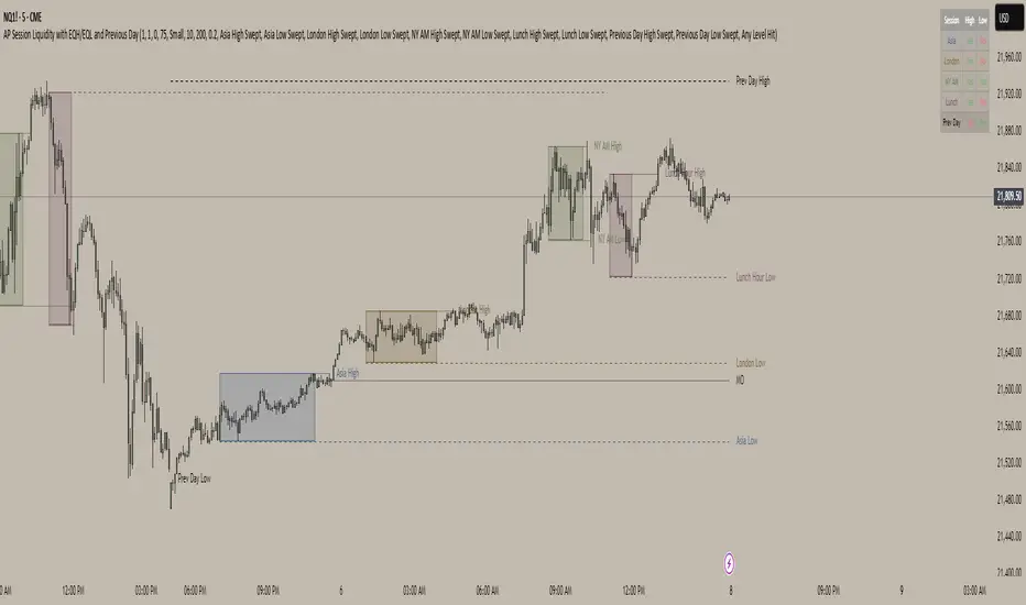
AP Session Liquidity with EQH/EQL and Previous DayThis indicator plots key intraday session highs and lows, along with essential market structure levels, to help traders identify areas of interest, potential liquidity zones, and high-probability trade setups. It includes the Asia Session High and Low (typically 00:00–08:00 UTC), London Session High and Low (08:00–12:00 UTC), New York AM Session High and Low (12:00–15:00 UTC), and New York Lunch High and Low (15:00–17:00 UTC). Additionally, it displays the Previous Day’s High and Low for context on recent price action, as well as automatically detected Equal Highs and Lows based on configurable proximity settings to highlight potential liquidity pools or engineered price levels. These session levels are widely used by institutional traders and are critical for analyzing market behavior during time-based volatility windows. Traders can use this indicator to anticipate breakouts, fakeouts, and reversals around session boundaries—such as liquidity grabs at Asia highs/lows before the London or New York sessions—or to identify key consolidation and expansion zones. Equal Highs and Lows serve as magnets for price, offering insight into potential stop hunts or inducement zones. This tool is ideal for day traders, scalpers, and smart money concept practitioners, and includes full customization for session timings, color schemes, line styles, and alert conditions. Whether you're trading price action, ICT concepts, or supply and demand, this indicator provides a powerful framework for intraday analysis.
5EMA_BB_ScalpingWhat?
In this forum we have earlier published a public scanner called 5EMA BollingerBand Nifty Stock Scanner , which is getting appreciated by the community. That works on top-40 stocks of NSE as a scanner.
Whereas this time, we have come up with the similar concept as a stand-alone indicator which can be applied for any chart, for any timeframe to reap the benifit of reversal trading.
How it works?
This is essentially a reversal/divergence trading strategy, based on a widely used strategy of Power-of-Stocks 5EMA.
To know the divergence from 5-EMA we just check if the high of the candle (on closing) is below the 5-EMA. Then we check if the closing is inside the Bollinger Band (BB). That's a Buy signal. SL: low of the candle, T: middle and higher BB.
Just opposite for selling. 5-EMA low should be above 5-EMA and closing should be inside BB (lesser than BB higher level). That's a Sell signal. SL: high of the candle, T: middle and lower BB.
Along with we compare the current bar's volume with the last-20 bar VWMA (volume weighted moving average) to determine if the volume is high or low.
Present bar's volume is compared with the previous bar's volume to know if it's rising or falling.
VWAP is also determined using `ta.vwap` built-in support of TradingView.
The Bolling Band width is also notified, along with whether it is rising or falling (comparing with previous candle).
What's special?
We love this reversal trading, as it offers many benifits over trend following strategies:
Risk to Reward (RR) is superior.
It _Does Hit_ stop losses, but the stop losses are tiny.
Means, althrough the Profit Factor looks Nahh , however due to superior RR, end of day it ended up in green.
When the day is sideways, it's difficult to trade in trending strategies. This sort of volatility, reversal strategies works better.
It's always tempting to go agaist the wind. Whole world is in Put/PE and you went opposite and enter a Call/CE. And turns out profitable! That's an amazing feeling, as a trader :)
How to trade using this?
* Put any chart
* Apply this screener from Indicators (shortcut to launch indicators is just type / in your keyboard).
* It will show you the Green up arrow when buy alert comes or red down arrow when sell comes. * Also on the top right it will show the latest signal with entry, SL and target.
Disclaimer
* This piece of software does not come up with any warrantee or any rights of not changing it over the future course of time.
* We are not responsible for any trading/investment decision you are taking out of the outcome of this indicator.

Asia Session Reversal Strategy GOLD (Full Version)📈 Asia Session Reversal Strategy (Gold/XAUUSD)
This indicator identifies high-probability reversal trades during the second hour of the Asia session (01:00–02:00 UTC) based on 30-minute candle bias. It:
Detects initial directional push and signals reversal trades on the 1-minute chart
Plots entry, stop-loss, and take-profit levels using a 3:1 reward-to-risk ratio
Includes real-time PnL tracking, daily auto-reset, and alert notifications for BUY/SELL setups
Ideal for scalpers and intraday traders focusing on Gold during consistent, high-liquidity session windows.
Custom Time Range Boxes + Fibs + ExtensionThis script draws two customizable time-range boxes per day, helping traders visualize key market sessions or activity windows. Each box is defined by start and end times that can be adjusted in the settings. You can also choose a custom color and extend the visual width of the box independently from the actual session time. Within each box, the indicator plots three Fibonacci levels: 0.3, 0.5, and 0.7. These levels are useful for identifying potential support, resistance, or retracement zones inside the session range. The script supports two separate time blocks, allowing you to track sessions like the New York Open and Power Hour simultaneously. All lines and boxes are drawn using bar_index for precision and control. The levels and box colors match for visual consistency. Perfect for intraday traders who want to track price behavior around key times. Clean, minimal, and performance-friendly — this tool adds clarity to your session-based strategy.
Lunar Cycle Tracker - (Moon + 3 Mercury Retrogrades)This script overlays the lunar and Mercury retrograde cycles directly onto your chart, helping traders visualize natural timing intervals that may influence market behavior.
Key Features:
🌑 New Moon & Full Moon Markers:
Vertical lines and labels indicate new and full moon events each month. You can fully customize their colors.
🌗 Last Quarter Moon Fill:
A soft pink background highlights the last quarter moon phase (from 7.4 days after the full moon to the next new moon).
🪐 Three Mercury Retrograde Zones:
Highlight up to three retrograde periods per year with customizable date inputs and background color. Great for spotting potential reversal or volatility windows.
Customization:
Moon event dates and colors
Manual input for Mercury retrograde periods (year, month, day)
Full compatibility with all timeframes (1H, 4H, daily, etc.)
Great for astro-cycle traders, Gann-based analysts, or anyone who respects time symmetry in the markets.
Fully customizable & works across all timeframes.
This tool was created by AngelArt as part of a larger astro-market model using lunar timing and planetary retrogrades for cycle-based market analysis.
Normalized MACD with RSI & Stoch RSI + SignalsNormalized MACD with RSI & Stoch RSI Indicator
Overview:
This indicator combines three popular momentum indicators (MACD, RSI, and Stochastic RSI) into a single cohesive, normalized view, making it easier for traders to interpret market momentum and potential buy/sell signals. It specifically addresses an important issue—the different scale ranges of indicators—by normalizing MACD values to match the 0–100 scale of RSI and Stochastic RSI.
Here’s a clear and concise description of your updated Pine Script indicator:
⸻
Normalized MACD with RSI & Stoch RSI Indicator
Overview:
This indicator combines three popular momentum indicators (MACD, RSI, and Stochastic RSI) into a single cohesive, normalized view, making it easier for traders to interpret market momentum and potential buy/sell signals. It specifically addresses an important issue—the different scale ranges of indicators—by normalizing MACD values to match the 0–100 scale of RSI and Stochastic RSI.
⸻
Key Components:
① MACD (Normalized):
• The Moving Average Convergence Divergence (MACD) originally has an unlimited numerical range.
• Normalization Method:
• Uses a custom tanh(x) function implemented directly in Pine Script:
\tanh(x) = \frac{e^{x}-e^{-x}}{e^{x}+e^{-x}}
• MACD values are scaled using this method to a range of 0–100, with the neutral line at exactly 50.
• Interpretation:
• Values above 50 indicate bullish momentum.
• Values below 50 indicate bearish momentum.
② RSI (Relative Strength Index):
• Measures market momentum on a 0–100 scale.
• Traditional RSI interpretation:
• Overbought conditions: RSI > 70–80.
• Oversold conditions: RSI < 30–20.
③ Stochastic RSI:
• Combines RSI and Stochastic Oscillator to give short-term, highly sensitive signals.
• Helps identify immediate market extremes:
• Above 80 → Short-term overbought.
• Below 20 → Short-term oversold.
⸻
How the Indicator Works:
• Visualization:
• All three indicators (Normalized MACD, RSI, Stochastic RSI) share the same 0–100 scale.
• Clear visual lines and reference levels:
• Midline at 50 indicates neutral momentum.
• Dashed lines at 20 and 80 clearly mark oversold/overbought zones.
• Trading Signals (Recommended approach):
• Bullish Signal (Potential Buy):
• Normalized MACD crosses above 50.
• RSI below or approaching oversold zone (below 30–20).
• Stochastic RSI below 20, indicating short-term oversold conditions.
• Bearish Signal (Potential Sell):
• Normalized MACD crosses below 50.
• RSI above or approaching overbought zone (above 70–80).
• Stochastic RSI above 80, indicating short-term overbought conditions.
⸻
Why Use This Indicator?
• Harmonized Signals:
Normalization of MACD significantly improves clarity and comparability with RSI and Stochastic RSI, providing a unified momentum picture.
• Intuitive Analysis:
Traders can rapidly and intuitively identify momentum shifts without needing multiple indicator windows.
• Improved Decision-Making:
Clear visual references and signals help reduce subjective interpretation, potentially improving trading outcomes.
⸻
Suggested Usage:
• Combine with traditional support
