Poly Cycle [Loxx]This is an example of what can be done by combining Legendre polynomials and analytic signals. I get a way of determining a smooth period and relative adaptive strength indicator without adding time lag.
This indicator displays the following:
The Least Squares fit of a polynomial to a DC subtracted time series - a best fit to a cycle.
The normalized analytic signal of the cycle (signal and quadrature).
The Phase shift of the analytic signal per bar.
The Period and HalfPeriod lengths, in bars of the current cycle.
A relative strength indicator of the time series over the cycle length. That is, adaptive relative strength over the cycle length.
The Relative Strength Indicator, is adaptive to the time series, and it can be smoothed by increasing the length of decreasing the number of degrees of freedom.
Other adaptive indicators based upon the period and can be similarly constructed.
There is some new math here, so I have broken the story up into 5 Parts:
Part 1:
Any time series can be decomposed into a orthogonal set of polynomials .
This is just math and here are some good references:
Legendre polynomials - Wikipedia, the free encyclopedia
Peter Seffen, "On Digital Smoothing Filters: A Brief Review of Closed Form Solutions and Two New Filter Approaches", Circuits Systems Signal Process, Vol. 5, No 2, 1986
I gave some thought to what should be done with this and came to the conclusion that they can be used for basic smoothing of time series. For the analysis below, I decompose a time series into a low number of degrees of freedom and discard the zero mode to introduce smoothing.
That is:
time series => c_1 t + c_2 t^2 ... c_Max t^Max
This is the cycle. By construction, the cycle does not have a zero mode and more physically, I am defining the "Trend" to be the zero mode.
The data for the cycle and the fit of the cycle can be viewed by setting
ShowDataAndFit = TRUE;
There, you will see the fit of the last bar as well as the time series of the leading edge of the fits. If you don't know what I mean by the "leading edge", please see some of the postings in . The leading edges are in grayscale, and the fit of the last bar is in color.
I have chosen Length = 17 and Degree = 4 as the default. I am simply making sure by eye that the fit is reasonably good and degree 4 is the lowest polynomial that can represent a sine-like wave, and 17 is the smallest length that lets me calculate the Phase Shift (Part 3 below) using the Hilbert Transform of width=7 (Part 2 below).
Depending upon the fit you make, you will capture different cycles in the data. A fit that is too "smooth" will not see the smaller cycles, and a fit that is too "choppy" will not see the longer ones. The idea is to use the fit to try to suppress the smaller noise cycles while keeping larger signal cycles.
Part 2:
Every time series has an Analytic Signal, defined by applying the Hilbert Transform to it. You can think of the original time series as amplitude * cosine(theta) and the transformed series, called the quadrature, can be thought of as amplitude * sine(theta). By taking the ratio, you can get the angle theta, and this is exactly what was done by John Ehlers in . It lets you get a frequency out of the time series under consideration.
Amazon.com: Rocket Science for Traders: Digital Signal Processing Applications (9780471405672): John F. Ehlers: Books
It helps to have more references to understand this. There is a nice article on Wikipedia on it.
Read the part about the discrete Hilbert Transform:
en.wikipedia.org
If you really want to understand how to go from continuous to discrete, look up this article written by Richard Lyons:
www.dspguru.com
In the indicator below, I am calculating the normalized analytic signal, which can be written as:
s + i h where i is the imagery number, and s^2 + h^2 = 1;
s= signal = cosine(theta)
h = Hilbert transformed signal = quadrature = sine(theta)
The angle is therefore given by theta = arctan(h/s);
The analytic signal leading edge and the fit of the last bar of the cycle can be viewed by setting
ShowAnalyticSignal = TRUE;
The leading edges are in grayscale fit to the last bar is in color. Light (yellow) is the s term, and Dark (orange) is the quadrature (hilbert transform). Note that for every bar, s^2 + h^2 = 1 , by construction.
I am using a width = 7 Hilbert transform, just like Ehlers. (But you can adjust it if you want.) This transform has a 7 bar lag. I have put the lag into the plot statements, so the cycle info should be quite good at displaying minima and maxima (extrema).
Part 3:
The Phase shift is the amount of phase change from bar to bar.
It is a discrete unitary transformation that takes s + i h to s + i h
explicitly, T = (s+ih)*(s -ih ) , since s *s + h *h = 1.
writing it out, we find that T = T1 + iT2
where T1 = s*s + h*h and T2 = s*h -h*s
and the phase shift is given by PhaseShift = arctan(T2/T1);
Alas, I have no reference for this, all I doing is finding the rotation what takes the analytic signal at bar to the analytic signal at bar . T is the transfer matrix.
Of interest is the PhaseShift from the closest two bars to the present, given by the bar and bar since I am using a width=7 Hilbert transform, bar is the earliest bar with an analytic signal.
I store the phase shift from bar to bar as a time series called PhaseShift. It basically gives you the (7-bar delayed) leading edge the amount of phase angle change in the series.
You can see it by setting
ShowPhaseShift=TRUE
The green points are positive phase shifts and red points are negative phase shifts.
On most charts, I have looked at, the indicator is mostly green, but occasionally, the stock "retrogrades" and red appears. This happens when the cycle is "broken" and the cycle length starts to expand as a trend occurs.
Part 4:
The Period:
The Period is the number of bars required to generate a sum of PhaseShifts equal to 360 degrees.
The Half-period is the number of bars required to generate a sum of phase shifts equal to 180 degrees. It is usually not equal to 1/2 of the period.
You can see the Period and Half-period by setting
ShowPeriod=TRUE
The code is very simple here:
Value1=0;
Value2=0;
while Value1 < bar_index and math.abs(Value2) < 360 begin
Value2 = Value2 + PhaseShift ;
Value1 = Value1 + 1;
end;
Period = Value1;
The period is sensitive to the input length and degree values but not overly so. Any insight on this would be appreciated.
Part 5:
The Relative Strength indicator:
The Relative Strength is just the current value of the series minus the minimum over the last cycle divided by the maximum - minimum over the last cycle, normalized between +1 and -1.
RelativeStrength = -1 + 2*(Series-Min)/(Max-Min);
It therefore tells you where the current bar is relative to the cycle. If you want to smooth the indicator, then extend the period and/or reduce the polynomial degree.
In code:
NewLength = floor(Period + HilbertWidth+1);
Max = highest(Series,NewLength);
Min = lowest(Series,NewLength);
if Max>Min then
Note that the variable NewLength includes the lag that comes from the Hilbert transform, (HilbertWidth=7 by default).
Conclusion:
This is an example of what can be done by combining Legendre polynomials and analytic signals to determine a smooth period without adding time lag.
________________________________
Changes in this one : instead of using true/false options for every single way to display, use Type parameter as following :
1. The Least Squares fit of a polynomial to a DC subtracted time series - a best fit to a cycle.
2. The normalized analytic signal of the cycle (signal and quadrature).
3. The Phase shift of the analytic signal per bar.
4. The Period and HalfPeriod lengths, in bars of the current cycle.
5. A relative strength indicator of the time series over the cycle length. That is, adaptive relative strength over the cycle length.
ค้นหาในสคริปต์สำหรับ "wave"

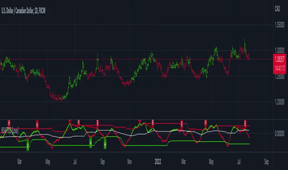
R-sqrd Adapt. Fisher Transform w/ D. Zones & Divs. [Loxx]The full name of this indicator is R-Squared Adaptive Fisher Transform w/ Dynamic Zones and Divergences. This is an R-squared adaptive Fisher transform with adjustable dynamic zones, signals, alerts, and divergences.
What is Fisher Transform?
The Fisher Transform is a technical indicator created by John F. Ehlers that converts prices into a Gaussian normal distribution.
The indicator highlights when prices have moved to an extreme, based on recent prices. This may help in spotting turning points in the price of an asset. It also helps show the trend and isolate the price waves within a trend.
What is R-squared Adaptive?
One tool available in forecasting the trendiness of the breakout is the coefficient of determination ( R-squared ), a statistical measurement.
The R-squared indicates linear strength between the security's price (the Y - axis) and time (the X - axis). The R-squared is the percentage of squared error that the linear regression can eliminate if it were used as the predictor instead of the mean value. If the R-squared were 0.99, then the linear regression would eliminate 99% of the error for prediction versus predicting closing prices using a simple moving average .
R-squared is used here to derive an r-squared value that is then modified by a user input "factor"
What are Dynamic Zones?
As explained in "Stocks & Commodities V15:7 (306-310): Dynamic Zones by Leo Zamansky, Ph .D., and David Stendahl"
Most indicators use a fixed zone for buy and sell signals. Here’ s a concept based on zones that are responsive to past levels of the indicator.
One approach to active investing employs the use of oscillators to exploit tradable market trends. This investing style follows a very simple form of logic: Enter the market only when an oscillator has moved far above or below traditional trading lev- els. However, these oscillator- driven systems lack the ability to evolve with the market because they use fixed buy and sell zones. Traders typically use one set of buy and sell zones for a bull market and substantially different zones for a bear market. And therein lies the problem.
Once traders begin introducing their market opinions into trading equations, by changing the zones, they negate the system’s mechanical nature. The objective is to have a system automatically define its own buy and sell zones and thereby profitably trade in any market — bull or bear. Dynamic zones offer a solution to the problem of fixed buy and sell zones for any oscillator-driven system.
An indicator’s extreme levels can be quantified using statistical methods. These extreme levels are calculated for a certain period and serve as the buy and sell zones for a trading system. The repetition of this statistical process for every value of the indicator creates values that become the dynamic zones. The zones are calculated in such a way that the probability of the indicator value rising above, or falling below, the dynamic zones is equal to a given probability input set by the trader.
To better understand dynamic zones, let's first describe them mathematically and then explain their use. The dynamic zones definition:
Find V such that:
For dynamic zone buy: P{X <= V}=P1
For dynamic zone sell: P{X >= V}=P2
where P1 and P2 are the probabilities set by the trader, X is the value of the indicator for the selected period and V represents the value of the dynamic zone.
The probability input P1 and P2 can be adjusted by the trader to encompass as much or as little data as the trader would like. The smaller the probability, the fewer data values above and below the dynamic zones. This translates into a wider range between the buy and sell zones. If a 10% probability is used for P1 and P2, only those data values that make up the top 10% and bottom 10% for an indicator are used in the construction of the zones. Of the values, 80% will fall between the two extreme levels. Because dynamic zone levels are penetrated so infrequently, when this happens, traders know that the market has truly moved into overbought or oversold territory.
Calculating the Dynamic Zones
The algorithm for the dynamic zones is a series of steps. First, decide the value of the lookback period t. Next, decide the value of the probability Pbuy for buy zone and value of the probability Psell for the sell zone.
For i=1, to the last lookback period, build the distribution f(x) of the price during the lookback period i. Then find the value Vi1 such that the probability of the price less than or equal to Vi1 during the lookback period i is equal to Pbuy. Find the value Vi2 such that the probability of the price greater or equal to Vi2 during the lookback period i is equal to Psell. The sequence of Vi1 for all periods gives the buy zone. The sequence of Vi2 for all periods gives the sell zone.
In the algorithm description, we have: Build the distribution f(x) of the price during the lookback period i. The distribution here is empirical namely, how many times a given value of x appeared during the lookback period. The problem is to find such x that the probability of a price being greater or equal to x will be equal to a probability selected by the user. Probability is the area under the distribution curve. The task is to find such value of x that the area under the distribution curve to the right of x will be equal to the probability selected by the user. That x is the dynamic zone.
Included:
Bar coloring
4 signal variations w/ alerts
Divergences w/ alerts
Loxx's Expanded Source Types
Trend Momentum Divergence (TMD)Shout out to Lazy Bear, Bunghole, and Trading View for script code for this make.
In this study you will have a visual representation of the strength and momentum of a trend and possibilities of where the market is heading. You can use the Blue and White momentum waves to spot divergences in a up oe down trend for potential reversals. When a green dot appears under the lower level with divergence then it is a indication that we should consider looking to buy. If the red dot appears over the upper level with divergence we should be looking to short/sell. The custom MFI indicator determines how much money is flowing into the market. If it is green that means money is flowing into the market and if it shows red it means that money is flowing out of the market. You can spot divergences in the money flow as well as the RSI. The Blue and Green lines from the RCI3line indicator are used for higher timeframe momentum based on current chart timeframe and we can see when they cross over.

Fisher Transform of MACD w/ Quantile Bands [Loxx]Fisher Transform of MACD w/ Quantile Bands is a Fisher Transform indicator with Quantile Bands that takes as it's source a MACD. The MACD has two different source inputs for fast and slow moving averages.
What is Fisher Transform?
The Fisher Transform is a technical indicator created by John F. Ehlers that converts prices into a Gaussian normal distribution.
The indicator highlights when prices have moved to an extreme, based on recent prices. This may help in spotting turning points in the price of an asset. It also helps show the trend and isolate the price waves within a trend.
What is Quantile Bands?
In statistics and the theory of probability, quantiles are cutpoints dividing the range of a probability distribution into contiguous intervals with equal probabilities, or dividing the observations in a sample in the same way. There is one less quantile than the number of groups created. Thus quartiles are the three cut points that will divide a dataset into four equal-size groups (cf. depicted example). Common quantiles have special names: for instance quartile, decile (creating 10 groups: see below for more). The groups created are termed halves, thirds, quarters, etc., though sometimes the terms for the quantile are used for the groups created, rather than for the cut points.
q-Quantiles are values that partition a finite set of values into q subsets of (nearly) equal sizes. There are q − 1 of the q-quantiles, one for each integer k satisfying 0 < k < q. In some cases the value of a quantile may not be uniquely determined, as can be the case for the median (2-quantile) of a uniform probability distribution on a set of even size. Quantiles can also be applied to continuous distributions, providing a way to generalize rank statistics to continuous variables. When the cumulative distribution function of a random variable is known, the q-quantiles are the application of the quantile function (the inverse function of the cumulative distribution function) to the values {1/q, 2/q, …, (q − 1)/q}.
What is MACD?
Moving average convergence divergence ( MACD ) is a trend-following momentum indicator that shows the relationship between two moving averages of a security’s price. The MACD is calculated by subtracting the 26-period exponential moving average ( EMA ) from the 12-period EMA .
Included:
Zero-line and signal cross options for bar coloring, signals, and alerts
Alerts
Signals
Loxx's Expanded Source Types
35+ moving average types

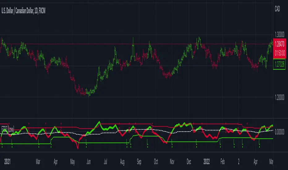
Fisher Transform w/ Dynamic Zones [Loxx]What is Fisher Transform?
The Fisher Transform is a technical indicator created by John F. Ehlers that converts prices into a Gaussian normal distribution.
The indicator highlights when prices have moved to an extreme, based on recent prices. This may help in spotting turning points in the price of an asset. It also helps show the trend and isolate the price waves within a trend.
What are Dynamic Zones?
As explained in "Stocks & Commodities V15:7 (306-310): Dynamic Zones by Leo Zamansky, Ph .D., and David Stendahl"
Most indicators use a fixed zone for buy and sell signals. Here’ s a concept based on zones that are responsive to past levels of the indicator.
One approach to active investing employs the use of oscillators to exploit tradable market trends. This investing style follows a very simple form of logic: Enter the market only when an oscillator has moved far above or below traditional trading lev- els. However, these oscillator- driven systems lack the ability to evolve with the market because they use fixed buy and sell zones. Traders typically use one set of buy and sell zones for a bull market and substantially different zones for a bear market. And therein lies the problem.
Once traders begin introducing their market opinions into trading equations, by changing the zones, they negate the system’s mechanical nature. The objective is to have a system automatically define its own buy and sell zones and thereby profitably trade in any market — bull or bear. Dynamic zones offer a solution to the problem of fixed buy and sell zones for any oscillator-driven system.
An indicator’s extreme levels can be quantified using statistical methods. These extreme levels are calculated for a certain period and serve as the buy and sell zones for a trading system. The repetition of this statistical process for every value of the indicator creates values that become the dynamic zones. The zones are calculated in such a way that the probability of the indicator value rising above, or falling below, the dynamic zones is equal to a given probability input set by the trader.
To better understand dynamic zones, let's first describe them mathematically and then explain their use. The dynamic zones definition:
Find V such that:
For dynamic zone buy: P{X <= V}=P1
For dynamic zone sell: P{X >= V}=P2
where P1 and P2 are the probabilities set by the trader, X is the value of the indicator for the selected period and V represents the value of the dynamic zone.
The probability input P1 and P2 can be adjusted by the trader to encompass as much or as little data as the trader would like. The smaller the probability, the fewer data values above and below the dynamic zones. This translates into a wider range between the buy and sell zones. If a 10% probability is used for P1 and P2, only those data values that make up the top 10% and bottom 10% for an indicator are used in the construction of the zones. Of the values, 80% will fall between the two extreme levels. Because dynamic zone levels are penetrated so infrequently, when this happens, traders know that the market has truly moved into overbought or oversold territory.
Calculating the Dynamic Zones
The algorithm for the dynamic zones is a series of steps. First, decide the value of the lookback period t. Next, decide the value of the probability Pbuy for buy zone and value of the probability Psell for the sell zone.
For i=1, to the last lookback period, build the distribution f(x) of the price during the lookback period i. Then find the value Vi1 such that the probability of the price less than or equal to Vi1 during the lookback period i is equal to Pbuy. Find the value Vi2 such that the probability of the price greater or equal to Vi2 during the lookback period i is equal to Psell. The sequence of Vi1 for all periods gives the buy zone. The sequence of Vi2 for all periods gives the sell zone.
In the algorithm description, we have: Build the distribution f(x) of the price during the lookback period i. The distribution here is empirical namely, how many times a given value of x appeared during the lookback period. The problem is to find such x that the probability of a price being greater or equal to x will be equal to a probability selected by the user. Probability is the area under the distribution curve. The task is to find such value of x that the area under the distribution curve to the right of x will be equal to the probability selected by the user. That x is the dynamic zone.
Included
3 signal types
Bar coloring
Alerts
Channels fill
Loxx's Expanded Source Types
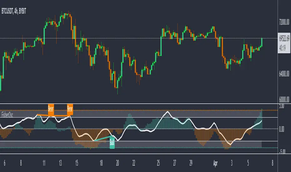
Fisher OscillatorThe indicator highlights when prices have moved to an extreme level, based on recent prices. This may help in spotting turning points in the price of an asset. It also helps show the trend and isolate the price waves within a trend.
VHF Adaptive ADXm [Loxx]VHF Adaptive ADXm is a variation of the ADX DI indicator with adaptive filtering using a vertical horizontal filter.
What is ADXm?
Unlike the traditional ADX indicator, where the ADX itself is plotted in absolute units and detection of the trend direction is hindered, this indicator clearly displays the positive and negative ADX half-waves (displayed as colored on the chart). And the DI+/- signals are displayed as their difference (gray).
The method of using this indicator is the same as the traditional one.
In addition, it displays the levels (dashed), above which the market is considered to be in a trend state. This level is usually set to approximately 20-25 percents--somewhat depends on the time frame it is used on.
What is VHF Adaptive Cycle?
Vertical Horizontal Filter (VHF) was created by Adam White to identify trending and ranging markets. VHF measures the level of trend activity, similar to ADX DI. Vertical Horizontal Filter does not, itself, generate trading signals, but determines whether signals are taken from trend or momentum indicators. Using this trend information, one is then able to derive an average cycle length.
Included:
Bar coloring
Alerts
Signal types: zero-line crosses, level crosses, or signal crosses

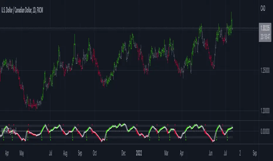
VHF Adaptive Fisher Transform [Loxx]VHF Adaptive Fisher Transform is an adaptive cycle Fisher Transform using a Vertical Horizontal Filter to calculate the volatility adjusted period.
What is VHF Adaptive Cycle?
Vertical Horizontal Filter (VHF) was created by Adam White to identify trending and ranging markets. VHF measures the level of trend activity, similar to ADX DI. Vertical Horizontal Filter does not, itself, generate trading signals, but determines whether signals are taken from trend or momentum indicators. Using this trend information, one is then able to derive an average cycle length.
What is Fisher Transform?
The Fisher Transform is a technical indicator created by John F. Ehlers that converts prices into a Gaussian normal distribution.
The indicator highlights when prices have moved to an extreme, based on recent prices. This may help in spotting turning points in the price of an asset. It also helps show the trend and isolate the price waves within a trend.
Included:
Zero-line and signal cross options for bar coloring
Customizable overbought/oversold thresh-holds
Alerts
Signals
CFB Adaptive Fisher Transform [Loxx]CFB Adaptive Fisher Transform is an adaptive cycle Fisher Transform using Jurik's Composite Fractal Behavior Algorithm to calculate the price-trend cycle period.
What is Composite Fractal Behavior (CFB)?
All around you mechanisms adjust themselves to their environment. From simple thermostats that react to air temperature to computer chips in modern cars that respond to changes in engine temperature, r.p.m.'s, torque, and throttle position. It was only a matter of time before fast desktop computers applied the mathematics of self-adjustment to systems that trade the financial markets.
Unlike basic systems with fixed formulas, an adaptive system adjusts its own equations. For example, start with a basic channel breakout system that uses the highest closing price of the last N bars as a threshold for detecting breakouts on the up side. An adaptive and improved version of this system would adjust N according to market conditions, such as momentum, price volatility or acceleration.
Since many systems are based directly or indirectly on cycles, another useful measure of market condition is the periodic length of a price chart's dominant cycle, (DC), that cycle with the greatest influence on price action.
The utility of this new DC measure was noted by author Murray Ruggiero in the January '96 issue of Futures Magazine. In it. Mr. Ruggiero used it to adaptive adjust the value of N in a channel breakout system. He then simulated trading 15 years of D-Mark futures in order to compare its performance to a similar system that had a fixed optimal value of N. The adaptive version produced 20% more profit!
This DC index utilized the popular MESA algorithm (a formulation by John Ehlers adapted from Burg's maximum entropy algorithm, MEM). Unfortunately, the DC approach is problematic when the market has no real dominant cycle momentum, because the mathematics will produce a value whether or not one actually exists! Therefore, we developed a proprietary indicator that does not presuppose the presence of market cycles. It's called CFB (Composite Fractal Behavior) and it works well whether or not the market is cyclic.
CFB examines price action for a particular fractal pattern, categorizes them by size, and then outputs a composite fractal size index. This index is smooth, timely and accurate
Essentially, CFB reveals the length of the market's trending action time frame. Long trending activity produces a large CFB index and short choppy action produces a small index value. Investors have found many applications for CFB which involve scaling other existing technical indicators adaptively, on a bar-to-bar basis.
What is Jurik Volty used in the Juirk Filter?
One of the lesser known qualities of Juirk smoothing is that the Jurik smoothing process is adaptive. "Jurik Volty" (a sort of market volatility ) is what makes Jurik smoothing adaptive. The Jurik Volty calculation can be used as both a standalone indicator and to smooth other indicators that you wish to make adaptive.
What is the Jurik Moving Average?
Have you noticed how moving averages add some lag (delay) to your signals? ... especially when price gaps up or down in a big move, and you are waiting for your moving average to catch up? Wait no more! JMA eliminates this problem forever and gives you the best of both worlds: low lag and smooth lines.
Ideally, you would like a filtered signal to be both smooth and lag-free. Lag causes delays in your trades, and increasing lag in your indicators typically result in lower profits. In other words, late comers get what's left on the table after the feast has already begun.
What is Fisher Transform?
The Fisher Transform is a technical indicator created by John F. Ehlers that converts prices into a Gaussian normal distribution.
The indicator highlights when prices have moved to an extreme, based on recent prices. This may help in spotting turning points in the price of an asset. It also helps show the trend and isolate the price waves within a trend.
Included:
Zero-line and signal cross options for bar coloring
Customizable overbought/oversold thresh-holds
Alerts
Signals

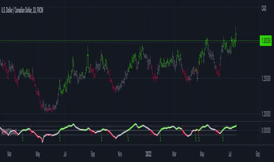
APA Adaptive Fisher Transform [Loxx]APA Adaptive Fisher Transform is an adaptive cycle Fisher Transform using Ehlers Autocorrelation Periodogram Algorithm to calculate the dominant cycle period.
What is an adaptive cycle, and what is Ehlers Autocorrelation Periodogram Algorithm?
From Ehlers' book Cycle Analytics for Traders Advanced Technical Trading Concepts by John F. Ehlers , 2013, page 135:
"Adaptive filters can have several different meanings. For example, Perry Kaufman’s adaptive moving average ( KAMA ) and Tushar Chande’s variable index dynamic average ( VIDYA ) adapt to changes in volatility . By definition, these filters are reactive to price changes, and therefore they close the barn door after the horse is gone.The adaptive filters discussed in this chapter are the familiar Stochastic , relative strength index ( RSI ), commodity channel index ( CCI ), and band-pass filter.The key parameter in each case is the look-back period used to calculate the indicator. This look-back period is commonly a fixed value. However, since the measured cycle period is changing, it makes sense to adapt these indicators to the measured cycle period. When tradable market cycles are observed, they tend to persist for a short while.Therefore, by tuning the indicators to the measure cycle period they are optimized for current conditions and can even have predictive characteristics.
The dominant cycle period is measured using the Autocorrelation Periodogram Algorithm. That dominant cycle dynamically sets the look-back period for the indicators. I employ my own streamlined computation for the indicators that provide smoother and easier to interpret outputs than traditional methods. Further, the indicator codes have been modified to remove the effects of spectral dilation.This basically creates a whole new set of indicators for your trading arsenal."
What is Fisher Transform?
The Fisher Transform is a technical indicator created by John F. Ehlers that converts prices into a Gaussian normal distribution.
The indicator highlights when prices have moved to an extreme, based on recent prices. This may help in spotting turning points in the price of an asset. It also helps show the trend and isolate the price waves within a trend.
Included:
Zero-line and signal cross options for bar coloring
Customizable overbought/oversold thresh-holds
Alerts
Signals
Phase Accumulation Adaptive Fisher Transform [Loxx]Phase Accumulation Adaptive Fisher Transform is an adaptive Fisher Transform using a modified version of Ehlers Phase Accumulation Cycle Period. This version of Phase Accumulation Cylce Period accepts as inputs: 1) total number of cycles you wish to inject into the calculation, this works as a multiplier so the higher this number, the longer the period output; 2) filter is to change the alpha value of the final smother before returning the period output.
What is the Phase Accumulation Cycle?
The phase accumulation method of computing the dominant cycle is perhaps the easiest to comprehend. In this technique, we measure the phase at each sample by taking the arctangent of the ratio of the quadrature component to the in-phase component. A delta phase is generated by taking the difference of the phase between successive samples. At each sample we can then look backwards, adding up the delta phases.When the sum of the delta phases reaches 360 degrees, we must have passed through one full cycle, on average.The process is repeated for each new sample.
The phase accumulation method of cycle measurement always uses one full cycle’s worth of historical data.This is both an advantage and a disadvantage.The advantage is the lag in obtaining the answer scales directly with the cycle period.That is, the measurement of a short cycle period has less lag than the measurement of a longer cycle period. However, the number of samples used in making the measurement means the averaging period is variable with cycle period. longer averaging reduces the noise level compared to the signal.Therefore, shorter cycle periods necessarily have a higher out- put signal-to-noise ratio.
What is Fisher Transform?
The Fisher Transform is a technical indicator created by John F. Ehlers that converts prices into a Gaussian normal distribution.
The indicator highlights when prices have moved to an extreme, based on recent prices. This may help in spotting turning points in the price of an asset. It also helps show the trend and isolate the price waves within a trend.
Included:
Zero-line and signal cross options for bar coloring
Customizable overbought/oversold thresh-holds
Alerts
Signals

Goertzel Cycle Period Adaptive Fisher Transform [Loxx]Goertzel Cycle Period Adaptive Fisher Transform is an adaptive Fisher Transform using the Goertzel Cycle Algorithm to derive length inputs.
What is Goertzel Cycle Algorithm?
Read here:
What is Fisher Transform?
The Fisher Transform is a technical indicator created by John F. Ehlers that converts prices into a Gaussian normal distribution.
The indicator highlights when prices have moved to an extreme, based on recent prices. This may help in spotting turning points in the price of an asset. It also helps show the trend and isolate the price waves within a trend.
Included:
Zero-line and signal cross options for bar coloring
Customizable overbought/oversold thresh-holds
Alerts
Signals
***Please note, the Goertzel Cycle Algorithm is processor heavy, so this indicator will take some time to load.

SweetSweetLucia: OnceADayUpdated:
3 Bar Typical Price (Offset 1 Bar)
1 Bar Open Price
Crosses are Opening Crossings of Typical Price
Squares are Intraday Close over Typical Price
Line Graph is Close, with colors
Short, Medium, and Large Fractal Wave Moving Averages
Format is Price Action
Thanks

Fake breakHi Traders,
I've developed an indicator which can detect fake-breaks on the chart.
In the following you'll find the definition of the fake break candles and also you will find how to recognize it on the chart with practical examples.
What is the fake break pattern?
Sometimes support and resistance lines broke with a full body and strong candles that gives us the idea of sharp movements on the chart but suddenly the next candle returns all the path of the previous candle. in this case we can say fake break is happening on the chart.
This indicator detect fake break patterns based on two criteria:
1. It uses AverageTrueRange indicator to measure the strength of the pattern.
2. The returning candle should engulf minimum 75% of the break candle.
This indicator plot 2 terms in the name of "FB-D" and "FB-U" that are abbreviations of the "Fake Break Down" and "Fake Break Up".
You can also set alerts to get notified when fake breakout happens on the chart.
Notice: This pattern is only acceptable in valid support and resistance zones and you can not rely on it everywhere on the chart (specially in the middle of the waves).
Notice: The source code of this indicator is open and you are allowed to use it on your scripts by mentioning the name of author.
Disclaimer: This is not a financial advice or any signal to buy or sell, the goal of developing such an indicator is to use for educational purposes.

APA-Adaptive, Ehlers Early Onset Trend [Loxx]APA-Adaptive, Ehlers Early Onset Trend is Ehlers Early Onset Trend but with Autocorrelation Periodogram Algorithm dominant cycle period input.
What is Ehlers Early Onset Trend?
The Onset Trend Detector study is a trend analyzing technical indicator developed by John F. Ehlers , based on a non-linear quotient transform. Two of Mr. Ehlers' previous studies, the Super Smoother Filter and the Roofing Filter, were used and expanded to create this new complex technical indicator. Being a trend-following analysis technique, its main purpose is to address the problem of lag that is common among moving average type indicators.
The Onset Trend Detector first applies the EhlersRoofingFilter to the input data in order to eliminate cyclic components with periods longer than, for example, 100 bars (default value, customizable via input parameters) as those are considered spectral dilation. Filtered data is then subjected to re-filtering by the Super Smoother Filter so that the noise (cyclic components with low length) is reduced to minimum. The period of 10 bars is a default maximum value for a wave cycle to be considered noise; it can be customized via input parameters as well. Once the data is cleared of both noise and spectral dilation, the filter processes it with the automatic gain control algorithm which is widely used in digital signal processing. This algorithm registers the most recent peak value and normalizes it; the normalized value slowly decays until the next peak swing. The ratio of previously filtered value to the corresponding peak value is then quotiently transformed to provide the resulting oscillator. The quotient transform is controlled by the K coefficient: its allowed values are in the range from -1 to +1. K values close to 1 leave the ratio almost untouched, those close to -1 will translate it to around the additive inverse, and those close to zero will collapse small values of the ratio while keeping the higher values high.
Indicator values around 1 signify uptrend and those around -1, downtrend.
What is an adaptive cycle, and what is Ehlers Autocorrelation Periodogram Algorithm?
From his Ehlers' book Cycle Analytics for Traders Advanced Technical Trading Concepts by John F. Ehlers , 2013, page 135:
"Adaptive filters can have several different meanings. For example, Perry Kaufman’s adaptive moving average ( KAMA ) and Tushar Chande’s variable index dynamic average ( VIDYA ) adapt to changes in volatility . By definition, these filters are reactive to price changes, and therefore they close the barn door after the horse is gone.The adaptive filters discussed in this chapter are the familiar Stochastic , relative strength index ( RSI ), commodity channel index ( CCI ), and band-pass filter.The key parameter in each case is the look-back period used to calculate the indicator. This look-back period is commonly a fixed value. However, since the measured cycle period is changing, it makes sense to adapt these indicators to the measured cycle period. When tradable market cycles are observed, they tend to persist for a short while.Therefore, by tuning the indicators to the measure cycle period they are optimized for current conditions and can even have predictive characteristics.
The dominant cycle period is measured using the Autocorrelation Periodogram Algorithm. That dominant cycle dynamically sets the look-back period for the indicators. I employ my own streamlined computation for the indicators that provide smoother and easier to interpret outputs than traditional methods. Further, the indicator codes have been modified to remove the effects of spectral dilation.This basically creates a whole new set of indicators for your trading arsenal."

DELAYED FIBOfibo delayed and real value wave design. Burada bandlar arası dalgalanmadan faydalanılmakta.
