Neural Network Buy and Sell SignalsTrend Architect Suite Lite - Neural Network Buy and Sell Signals
Advanced AI-Powered Signal Scoring
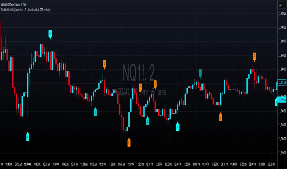
This indicator provides neural network market analysis on buy and sell signals designed for scalpers and day traders who use 30s to 5m charts. Signals are generated based on an ATR system and then filtered and scored using an advanced AI-driven system.
Features
Neural Network Signal Engine
5-Layer Deep Learning analysis combining market structure, momentum, and market state detection
AI-based Letter Grade Scoring (A+ through F) for instant signal quality assessment
Normalized Input Processing with Z-score standardization and outlier clipping
Real-time Signal Evaluation using 5 market dimensions
Advanced Candle Types
Standard Candlesticks - Raw price action
Heikin Ashi - Trend smoothing and noise reduction
Linear Regression - Mathematical trend visualization
Independent Signal vs Display - Calculate signals on one type, display another
Key Settings
Signal Configuration
- Signal Trigger Sensitivity (Default: 1.7) - Controls signal frequency vs quality
- Stop Loss ATR Multiplier (Default: 1.5) - Risk management sizing
- Signal Candle Type (Default: Candlesticks) - Data source for signal calculations
- Display Candle Type (Default: Linear Regression) - Visual candle display
Display Options
- Signal Distance (Default: 1.35 ATR) - Label positioning from price
- Label Size (Default: Medium) - Optimal readability
Trading Applications
Scalping
- Fast pace signal detection with quality filtering
- ATR-based stop management prevents signal overlap
- Neural network attempts to reduces false signals in choppy markets
Day Trading
- Multi-timeframe compatible with adaptation settings
- Clear trend visualization with Linear Regression candles
- Support/resistance integration for better entries/exits
Signal Filtering
- Use A+/A grades for highest probability setups
- B grades for confirmation in trending markets
- C-F grades help identify market uncertainty
Why Choose Trend Architect Lite?
No Lag - Real-time neural network processing
No Repainting - Signals appear and stay fixed
Clean Charts - Focus on price action, not indicators
Smart Filtering - AI reduces noise and false signals
Flexible and customizable - Works across all timeframes and instruments
Compatibility
- All Timeframes - 1m to Monthly charts
- All Instruments - Forex, Crypto, Stocks, Futures, Indices
Risk Disclaimer
This indicator is a tool for technical analysis and should not be used as the sole basis for trading decisions. Past performance does not guarantee future results. Always use proper risk management and never risk more than you can afford to lose.
ค้นหาในสคริปต์สำหรับ "deep股票代码"
FEDFUNDS Rate Divergence Oscillator [BackQuant]FEDFUNDS Rate Divergence Oscillator
1. Concept and Rationale
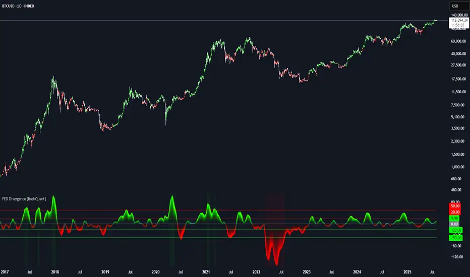
The United States Federal Funds Rate is the anchor around which global dollar liquidity and risk-free yield expectations revolve. When the Fed hikes, borrowing costs rise, liquidity tightens and most risk assets encounter head-winds. When it cuts, liquidity expands, speculative appetite often recovers. Bitcoin, a 24-hour permissionless asset sometimes described as “digital gold with venture-capital-like convexity,” is particularly sensitive to macro-liquidity swings.
The FED Divergence Oscillator quantifies the behavioural gap between short-term monetary policy (proxied by the effective Fed Funds Rate) and Bitcoin’s own percentage price change. By converting each series into identical rate-of-change units, subtracting them, then optionally smoothing the result, the script produces a single bounded-yet-dynamic line that tells you, at a glance, whether Bitcoin is outperforming or underperforming the policy backdrop—and by how much.
2. Data Pipeline
• Fed Funds Rate – Pulled directly from the FRED database via the ticker “FRED:FEDFUNDS,” sampled at daily frequency to synchronise with crypto closes.
• Bitcoin Price – By default the script forces a daily timeframe so that both series share time alignment, although you can disable that and plot the oscillator on intraday charts if you prefer.
• User Source Flexibility – The BTC series is not hard-wired; you can select any exchange-specific symbol or even swap BTC for another crypto or risk asset whose interaction with the Fed rate you wish to study.
3. Math under the Hood
(1) Rate of Change (ROC) – Both the Fed rate and BTC close are converted to percent return over a user-chosen lookback (default 30 bars). This means a cut from 5.25 percent to 5.00 percent feeds in as –4.76 percent, while a climb from 25 000 to 30 000 USD in BTC over the same window converts to +20 percent.
(2) Divergence Construction – The script subtracts the Fed ROC from the BTC ROC. Positive values show BTC appreciating faster than policy is tightening (or falling slower than the rate is cutting); negative values show the opposite.
(3) Optional Smoothing – Macro series are noisy. Toggle “Apply Smoothing” to calm the line with your preferred moving-average flavour: SMA, EMA, DEMA, TEMA, RMA, WMA or Hull. The default EMA-25 removes day-to-day whips while keeping turning points alive.
(4) Dynamic Colour Mapping – Rather than using a single hue, the oscillator line employs a gradient where deep greens represent strong bullish divergence and dark reds flag sharp bearish divergence. This heat-map approach lets you gauge intensity without squinting at numbers.
(5) Threshold Grid – Five horizontal guides create a structured regime map:
• Lower Extreme (–50 pct) and Upper Extreme (+50 pct) identify panic capitulations and euphoria blow-offs.
• Oversold (–20 pct) and Overbought (+20 pct) act as early warning alarms.
• Zero Line demarcates neutral alignment.
4. Chart Furniture and User Interface
• Oscillator fill with a secondary DEMA-30 “shader” offers depth perception: fat ribbons often precede high-volatility macro shifts.
• Optional bar-colouring paints candles green when the oscillator is above zero and red below, handy for visual correlation.
• Background tints when the line breaches extreme zones, making macro inflection weeks pop out in the replay bar.
• Everything—line width, thresholds, colours—can be customised so the indicator blends into any template.
5. Interpretation Guide
Macro Liquidity Pulse
• When the oscillator spends weeks above +20 while the Fed is still raising rates, Bitcoin is signalling liquidity tolerance or an anticipatory pivot view. That condition often marks the embryonic phase of major bull cycles (e.g., March 2020 rebound).
• Sustained prints below –20 while the Fed is already dovish indicate risk aversion or idiosyncratic crypto stress—think exchange scandals or broad flight to safety.
Regime Transition Signals
• Bullish cross through zero after a long sub-zero stint shows Bitcoin regaining upward escape velocity versus policy.
• Bearish cross under zero during a hiking cycle tells you monetary tightening has finally started to bite.
Momentum Exhaustion and Mean-Reversion
• Touches of +50 (or –50) come rarely; they are statistically stretched events. Fade strategies either taking profits or hedging have historically enjoyed positive expectancy.
• Inside-bar candlestick patterns or lower-timeframe bearish engulfings simultaneously with an extreme overbought print make high-probability short scalp setups, especially near weekly resistance. The same logic mirrors for oversold.
Pair Trading / Relative Value
• Combine the oscillator with spreads like BTC versus Nasdaq 100. When both the FED Divergence oscillator and the BTC–NDQ relative-strength line roll south together, the cross-asset confirmation amplifies conviction in a mean-reversion short.
• Swap BTC for miners, altcoins or high-beta equities to test who is the divergence leader.
Event-Driven Tactics
• FOMC days: plot the oscillator on an hourly chart (disable ‘Force Daily TF’). Watch for micro-structural spikes that resolve in the first hour after the statement; rapid flips across zero can front-run post-FOMC swings.
• CPI and NFP prints: extremes reached into the release often mean positioning is one-sided. A reversion toward neutral in the first 24 hours is common.
6. Alerts Suite
Pre-bundled conditions let you automate workflows:
• Bullish / Bearish zero crosses – queue spot or futures entries.
• Standard OB / OS – notify for first contact with actionable zones.
• Extreme OB / OS – prime time to review hedges, take profits or build contrarian swing positions.
7. Parameter Playground
• Shorten ROC Lookback to 14 for tactical traders; lengthen to 90 for macro investors.
• Raise extreme thresholds (for example ±80) when plotting on altcoins that exhibit higher volatility than BTC.
• Try HMA smoothing for responsive yet smooth curves on intraday charts.
• Colour-blind users can easily swap bull and bear palette selections for preferred contrasts.
8. Limitations and Best Practices
• The Fed Funds series is step-wise; it only changes on meeting days. Rapid BTC oscillations in between may dominate the calculation. Keep that perspective when interpreting very high-frequency signals.
• Divergence does not equal causation. Crypto-native catalysts (ETF approvals, hack headlines) can overwhelm macro links temporarily.
• Use in conjunction with classical confirmation tools—order-flow footprints, market-profile ledges, or simple price action to avoid “pure-indicator” traps.
9. Final Thoughts
The FEDFUNDS Rate Divergence Oscillator distills an entire macro narrative monetary policy versus risk sentiment into a single colourful heartbeat. It will not magically predict every pivot, yet it excels at framing market context, spotting stretches and timing regime changes. Treat it as a strategic compass rather than a tactical sniper scope, combine it with sound risk management and multi-factor confirmation, and you will possess a robust edge anchored in the world’s most influential interest-rate benchmark.
Trade consciously, stay adaptive, and let the policy-price tension guide your roadmap.
Simple 5 Moving Averages 5 MAs - Shubhashish DixitEnjoy the 5 Moving Average to Support your analysis deeper

Advanced ICT Theory - A-ICT📊 Advanced ICT Theory (A-ICT): The Institutional Manipulation Detector
Are you tired of being the liquidity? Stop chasing shadows and start tracking the architects of price movement.
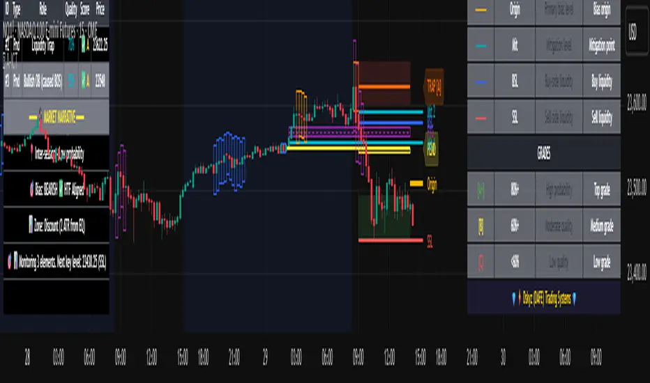
This is not another lagging indicator. This is a complete framework for viewing the market through the lens of institutional traders. Advanced ICT Theory (A-ICT) is an all-in-one, military-grade analysis engine designed to decode the complex language of "Smart Money." It automates the core tenets of Inner Circle Trader (ICT) methodology, moving beyond simple patterns to build a dynamic, real-time narrative of market manipulation, liquidity engineering, and institutional order flow.
AIT provides a living blueprint of the market, identifying high-probability zones, tracking structural shifts, and scoring the quality of setups with a sophisticated, multi-factor algorithm. This is your X-ray into the market's true intentions.
🔬 THE CORE ENGINE: DECODING THE THEORY & FORMULAS
A-ICT is built upon a sophisticated, multi-layered logic system that interprets price action as a story of cause and effect. It does not guess; it confirms. Here is the foundational theory that drives the engine:
1. Market Structure: The Blueprint of Trend
The script first establishes a deep understanding of the market's skeleton through multi-level pivot analysis. It uses ta.pivothigh and ta.pivotlow to identify significant swing points.
Internal Structure (iBOS): Minor swings that show the short-term order flow. A break of internal structure is the first whisper of a potential shift.
External Structure (eBOS): Major swing points that define the primary trend. A confirmed break of external structure is a powerful statement of trend continuation. AIT validates this with optional Volume Confirmation (volume > volumeSMA * 1.2) and Candle Confirmation to ensure the break is driven by institutional force, not just a random spike.
Change of Character (CHoCH): This is the earthquake. A CHoCH occurs when a confirmed eBOS happens against the prevailing trend (e.g., a bearish eBOS in a clear uptrend). A-ICT flags this immediately, as it is the strongest signal that the primary trend is under threat of reversal.
2. Liquidity Engineering: The Fuel of the Market
Institutions don't buy into strength; they buy into weakness. They need liquidity. A-ICT maps these liquidity pools with forensic precision:
Buyside & Sellside Liquidity (BSL/SSL): Using ta.highest and ta.lowest, AIT identifies recent highs and lows where clusters of stop-loss orders (liquidity) are resting. These are institutional targets.
Liquidity Sweeps: This is the "manipulation" part of the detector. AIT has a specific formula to detect a sweep: high > bsl and close < bsl . This signifies that institutions pushed price just high enough to trigger buy-stops before aggressively selling—a classic "stop hunt." This event dramatically increases the quality score of subsequent patterns.
3. The Element Lifecycle: From Potential to Power
This is the revolutionary heart of A-ICT. Zones are not static; they have a lifecycle. AIT tracks this with its dynamic classification engine.
Phase 1: PENDING (Yellow): The script identifies a potential zone of interest based on a specific candle formation (a "displacement"). It is marked as "Pending" because its true nature is unknown. It is a question.
Phase 2: CLASSIFICATION: After the zone is created, AIT watches what happens next. The zone's identity is defined by its actions:
ORDER BLOCK (Blue): The highest-grade element. A zone is classified as an Order Block if it directly causes a Break of Structure (BOS) . This is the footprint of institutions entering the market with enough force to validate the new trend direction.
TRAP ZONE (Orange): A zone is classified as a Trap Zone if it is directly involved in a Liquidity Sweep . This indicates the zone was used to engineer liquidity, setting a "trap" for retail traders before a reversal.
REVERSAL / S&R ZONE (Green): If a zone is not powerful enough to cause a BOS or a major sweep, but still serves as a pivot point, it's classified as a general support/resistance or reversal zone.
4. Market Inefficiencies: Gaps in the Matrix
Fair Value Gaps (FVG): AIT detects FVGs—a 3-bar pattern indicating an imbalance—with a strict formula: low > high (for a bullish FVG) and gapSize > atr14 * 0.5. This ensures only significant, volatile gaps are shown. An FVG co-located with an Order Block is a high-confluence setup.
5. Premium & Discount: The Law of Value
Institutions buy at wholesale (Discount) and sell at retail (Premium). AIT uses a pdLookback to define the current dealing range and divides it into three zones: Premium (sell zone), Discount (buy zone), and Equilibrium. An element's quality score is massively boosted if it aligns with this principle (e.g., a bullish Order Block in a Discount zone).
⚙️ THE CONTROL PANEL: A COMPLETE GUIDE TO THE INPUTS MENU
Every setting is a lever, allowing you to tune the AIT engine to your exact specifications. Master these to unlock the script's full potential.
🎯 A-ICT Detection Engine
Min Displacement Candles: Controls the sensitivity of element detection. How it works: It defines the number of subsequent candles that must be "inside" a large parent candle. Best practice: Use 2-3 for a balanced view on most timeframes. A higher number (4-5) will find only major, more significant zones, ideal for swing trading. A lower number (1) is highly sensitive, suitable for scalping.
Mitigation Method: Defines when a zone is considered "used up" or mitigated. How it works: Cross triggers as soon as price touches the zone's boundary. Close requires a candle to fully close beyond it. Best practice: Cross is more responsive for fast-moving markets. Close is more conservative and helps filter out fake-outs caused by wicks, making it safer for confirmations.
Min Element Size (ATR): A crucial noise filter. How it works: It requires a detected zone to be at least this multiple of the Average True Range (ATR). Best practice: Keep this around 0.5. If you see too many tiny, irrelevant zones, increase this value to 0.8 or 1.0. If you feel the script is missing smaller but valid zones, decrease it to 0.3.
Age Threshold & Pending Timeout: These manage visual clutter. How they work: Age Threshold removes old, mitigated elements after a set number of bars. Pending Timeout removes a "Pending" element if it isn't classified within a certain window. Best practice: The default settings are optimized. If your chart feels cluttered, reduce the Age Threshold. If pending zones disappear too quickly, increase the Pending Timeout.
Min Quality Threshold: Your primary visual filter. How it works: It hides all elements (boxes, lines, labels) that do not meet this minimum quality score (0-100). Best practice: Start with the default 30. To see only A- or B-grade setups, increase this to 60 or 70 for an exceptionally clean, high-probability view.
🏗️ Market Structure
Lookbacks (Internal, External, Major): These define the sensitivity of the trend analysis. How they work: They set the number of bars to the left and right for pivot detection. Best practice: Use smaller values for Internal (e.g., 3) to see minor structure and larger values for External (e.g., 10-15) to map the main trend. For a macro, long-term view, increase the Major Swing Lookback.
Require Volume/Candle Confirmation: Toggles for quality control on BOS/CHoCH signals. Best practice: It is highly recommended to keep these enabled. Disabling them will result in more structure signals, but many will be false alarms. They are your filter against market noise.
... (Continue this detailed breakdown for every single input group: Display Configuration, Zones Style, Levels Appearance, Colors, Dashboards, MTF, Liquidity, Premium/Discount, Sessions, and IPDA).
📊 THE INTELLIGENCE DASHBOARDS: YOUR COMMAND CENTER
The dashboards synthesize all the complex analysis into a simple, actionable intelligence briefing.
Main Dashboard (Bottom Right)
ICT Metrics & Breakdown: This is your statistical overview. Total Elements shows how much structure the script is tracking. High Quality instantly tells you if there are any A/B grade setups nearby. Unmitigated vs. Mitigated shows the balance of fresh opportunities versus resolved price action. The breakdown by Order Blocks, Trap Zones, etc., gives you a quick read on the market's recent character.
Structure & Market Context: This is your core bias. Order Flow tells you the current script-determined trend. Last BOS shows you the most recent structural event. CHoCH Active is a critical warning. HTF Bias shows if you are aligned with the higher timeframe—the checkmark (✓) for alignment is one of the most important confluence factors.
Smart Money Flow: A volume-based sentiment gauge. Net Flow shows the raw buying vs. selling pressure, while the Bias provides an interpretation (e.g., "STRONG BULLISH FLOW").
Key Guide (Large Dashboard only): A built-in legend so you never have to guess. It defines every pattern, structure type, and special level visually.
📖 Narrative Dashboard (Bottom Left)
This is the "story" of the market, updated in real-time. It's designed to build your trading thesis.
Recent Elements Table: A live list of the most recent, high-quality setups. It displays the Type , its Narrative Role (e.g., "Bullish OB caused BOS"), its raw Quality percentage, and its final Trade Score grade. This is your at-a-glance opportunity scanner.
Market Narrative Section: This is the soul of A-ICT. It combines all data points into a human-readable story:
📍 Current Phase: Tells you if you are in a high-volatility Killzone or a consolidation phase like the Asian Range.
🎯 Bias & Alignment: Your primary direction, with a clear indicator of HTF alignment or conflict.
🔗 Events: A causal sequence of recent events, like "💧 Sell-side liquidity swept →
📊 Bullish BOS → 🎯 Active Order Block".
🎯 Next Expectation: The script's logical conclusion. It provides a specific, forward-looking hypothesis, such as "📉 Pullback expected to bullish OB at 1.2345 before continuation up."
🎨 READING THE BATTLEFIELD: A VISUAL INTERPRETATION GUIDE
Every color and line is a piece of information. Learn to read them together to see the full picture.
The Core Zones (Boxes):
Blue Box (Order Block): Highest probability zone for trend continuation. Look for entries here.
Orange Box (Trap Zone): A manipulation footprint. Expect a potential reversal after price interacts with this zone.
Green Box (Reversal/S&R): A standard pivot area. A good reference point but requires more confluence.
Purple Box (FVG): A market imbalance. Acts as a magnet for price. An FVG inside an Order Block is an A+ confluence.
The Structural Lines:
Green/Red Line (eBOS): Confirms the trend direction. A break above the green line is bullish; a break below the red line is bearish.
Thick Orange Line (CHoCH): WARNING. The previous trend is now in question. The market character has changed.
Blue/Red Lines (BSL/SSL): Liquidity targets. Expect price to gravitate towards these lines. A dotted line with a checkmark (✓) means the liquidity has been "swept" or "purged."
How to Synthesize: The magic is in the confluence. A perfect setup might look like this: Price sweeps below a red SSL line , enters a green Discount Zone during the NY Killzone , and forms a blue Order Block which then causes a green eBOS . This sequence, visible at a glance, is the story of a high-probability long setup.
🔧 THE ARCHITECT'S VISION: THE DEVELOPMENT JOURNEY
A-ICT was forged from the frustration of using lagging indicators in a market that is forward-looking. Traditional tools are reactive; they tell you what happened. The vision for A-ICT was to create a proactive engine that could anticipate institutional behavior by understanding their objectives: liquidity and efficiency. The development process was centered on creating a "lifecycle" for price patterns—the idea that a zone's true meaning is only revealed by its consequence. This led to the post-breakout classification system and the narrative-building engine. It's designed not just to show you patterns, but to tell you their story.
⚠️ RISK DISCLAIMER & BEST PRACTICES
Advanced ICT Theory (A-ICT) is a professional-grade analytical tool and does not provide financial advice or direct buy/sell signals. Its analysis is based on historical price action and probabilities. All forms of trading involve substantial risk. Past performance is not indicative of future results. Always use this tool as part of a comprehensive trading plan that includes your own analysis and a robust risk management strategy. Do not trade based on this indicator alone.
観の目つよく、見の目よわく
"Kan no me tsuyoku, ken no me yowaku"
— Miyamoto Musashi, The Book of Five Rings
English: "Perceive that which cannot be seen with the eye."
— Dskyz, Trade with insight. Trade with anticipation.
Volume Footprint Anomaly Scanner [PhenLabs]📊 PhenLabs - Volume Footprint Anomaly Scanner (VFAS)
Version: PineScript™ v6
📌 Description
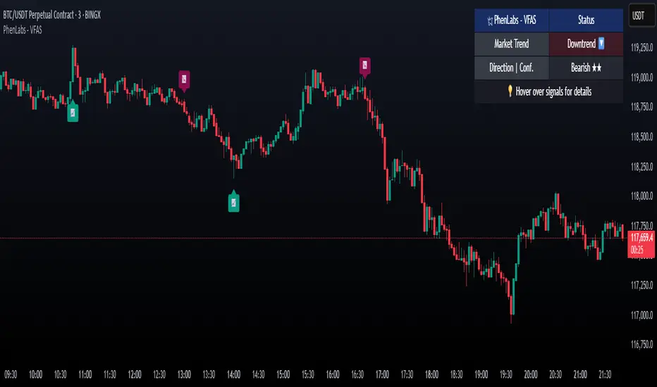
The PhenLabs Volume Footprint Anomaly Scanner (VFAS) is an advanced Pine Script indicator designed to detect and highlight significant imbalances in buying and selling pressure within individual price bars. By analyzing a calculated "Delta" – the net difference between estimated buy and sell volume – and employing statistical Z-score analysis, VFAS pinpoints moments when buying or selling activity becomes unusually dominant. This script was created not in hopes of creating a "Buy and Sell" indicator but rather providing the user with a more in-depth insight into the intrabar volume delta and how it can fluctuate in unusual ways, leading to anomalies that can be capitalized on.
This indicator helps traders identify high-conviction points where strong market participants are active, signaling potential shifts in momentum or continuation of a trend. It aims to provide a clearer understanding of underlying market dynamics, allowing for more informed decision-making in various trading strategies, from identifying entry points to confirming trend strength.
🚀 Points of Innovation
● Z-Score for Delta Analysis : Utilizes statistical Z-scores to objectively identify statistically significant anomalies in buying/selling pressure, moving beyond simple, arbitrary thresholds.
● Dynamic Confidence Scoring : Assigns a multi-star confidence rating (1-4 stars) to each signal, factoring in high volume, trend alignment, and specific confirmation criteria, providing a nuanced view of signal strength.
● Integrated Trend Filtering : Offers an optional Exponential Moving Average (EMA)-based trend filter to ensure signals align with the broader market direction, reducing false positives in ranging markets.
● Strict Confirmation Logic : Implements specific confirmation criteria for higher-confidence signals, including price action and a time-based gap from previous signals, enhancing reliability.
● Intuitive Info Dashboard : Provides a real-time summary of market trend and the latest signal's direction and confidence directly on the chart, streamlining information access.
🔧 Core Components
● Core Delta Engine : Estimates the net buying/selling pressure (bar Delta) by analyzing price movement within each bar relative to volume. It also calculates average volume to identify bars with unusually high activity.
● Anomaly Detection (Z-Score) : Computes the Z-score for the current bar's Delta, indicating how many standard deviations it is from its recent average. This statistical measure is central to identifying significant anomalies.
● Trend Filter : Utilizes a dual Exponential Moving Average (EMA) cross-over system to define the prevailing market trend (uptrend, downtrend, or range), providing contextual awareness.
● Signal Processing & Confidence Algorithm : Evaluates anomaly conditions against trend filters and confirmation rules, then calculates a dynamic confidence score to produce actionable, contextualized signal information.
🔥 Key Features
● Advanced Delta Anomaly Detection : Pinpoints bars with exceptionally high buying or selling pressure, indicating potential institutional activity or strong market conviction.
● Multi-Factor Confidence Scoring : Each signal comes with a 1-4 star rating, clearly communicating its reliability based on high volume, trend alignment, and specific confirmation criteria.
● Optional Trend Alignment : Users can choose to filter signals, so only those aligned with the prevailing EMA-defined trend are displayed, enhancing signal quality.
● Interactive Signal Labels : Displays compact labels on the chart at anomaly points, offering detailed tooltips upon hover, including signal type, direction, confidence, and contextual information.
● Customizable Bar Colors : Visually highlights bars with Delta anomalies, providing an immediate visual cue for strong buying or selling activity.
● Real-time Info Dashboard : A clean, customizable dashboard shows the current market trend and details of the latest detected signal, keeping key information accessible at a glance.
● Configurable Alerts : Set up alerts for bullish or bearish Delta anomalies to receive real-time notifications when significant market pressure shifts occur.
🎨 Visualization
Signal Labels :
* Placed at the top/bottom of anomaly bars, showing a "📈" (bullish) or "📉" (bearish) icon.
* Tooltip: Hovering over a label reveals detailed information: Signal Type (e.g., "Delta Anomaly"), Direction, Confidence (e.g., "★★★☆"), and a descriptive explanation of the anomaly.
* Interpretation: Clearly marks actionable signals and provides deep insights without cluttering the chart, enabling quick assessment of signal strength and context.
● Info Dashboard :
* Located at the top-right of the chart, providing a clean summary.
* Displays: "PhenLabs - VFAS" header, "Market Trend" (Uptrend/Downtrend/Range with color-coded status), and "Direction | Conf." (showing the last signal's direction and star confidence).
* Optional "💡 Hover over signals for details" reminder.
* Interpretation: A concise, real-time summary of the market's pulse and the most recent high-conviction event, helping traders stay informed at a glance.
📖 Usage Guidelines
Setting Categories
⚙️ Core Delta & Volume Engine
● Minimum Volume Lookback (Bars)
○ Default: 9
○ Range: Integer (e.g., 5-50)
○ Description: Defines the number of preceding bars used to calculate the average volume and delta. Bars with volume below this average won't be considered for high-volume signals. A shorter lookback is more reactive to recent changes, while a longer one provides a smoother average.
📈 Anomaly Detection Settings
Delta Z-Score Anomaly Threshold
○ Default: 2.5
○ Range: Float (e.g., 1.0-5.0+)
○ Description: The number of standard deviations from the mean that a bar's delta must exceed to be considered a significant anomaly. A higher threshold means fewer, but potentially stronger, signals. A lower threshold will generate more signals, which might include less significant events. Experiment to find the optimal balance for your trading style.
🔬 Context Filters
Enable Trend Filter
○ Default: False
○ Range: Boolean (True/False)
○ Description: When enabled, signals will only be generated if they align with the current market trend as determined by the EMAs (e.g., only bullish signals in an uptrend, bearish in a downtrend). This helps to filter out counter-trend noise.
● Trend EMA Fast
○ Default: 50
○ Range: Integer (e.g., 10-100)
○ Description: The period for the faster Exponential Moving Average used in the trend filter. In combination with the slow EMA, it defines the trend direction.
● Trend EMA Slow
○ Default: 200
○ Range: Integer (e.g., 100-400)
○ Description: The period for the slower Exponential Moving Average used in the trend filter. The relationship between the fast and slow EMA determines if the market is in an uptrend (fast > slow) or downtrend (fast < slow).
🎨 Visual & UI Settings
● Show Info Dashboard
○ Default: True
○ Range: Boolean (True/False)
○ Description: Toggles the visibility of the dashboard on the chart, which provides a summary of market trend and the last detected signal.
● Show Dashboard Tooltip
○ Default: True
○ Range: Boolean (True/False)
○ Description: Toggles a reminder message in the dashboard to hover over signal labels for more detailed information.
● Show Delta Anomaly Bar Colors
○ Default: True
○ Range: Boolean (True/False)
○ Description: Enables or disables the coloring of bars based on their delta direction and whether they represent a significant anomaly.
● Show Signal Labels
○ Default: True
○ Range: Boolean (True/False)
○ Description: Controls the visibility of the “📈” or “📉” labels that appear on the chart when a delta anomaly signal is generated.
🔔 Alert Settings
Alert on Delta Anomaly
○ Default: True
○ Range: Boolean (True/False)
○ Description: When enabled, this setting allows you to set up alerts in TradingView that will trigger whenever a new bullish or bearish delta anomaly is detected.
✅ Best Use Cases
Early Trend Reversal / Continuation Detection: Identify strong surges of buying/selling pressure at key support/resistance levels that could indicate a reversal or the continuation of a strong move.
● Confirmation of Breakouts: Use high-confidence delta anomalies to confirm the validity of price breakouts, indicating strong conviction behind the move.
● Entry and Exit Points: Pinpoint precise entry opportunities when anomalies align with your trading strategy, or identify potential exhaustion signals for exiting trades.
● Scalping and Day Trading: The indicator’s sensitivity to intraday buying/selling imbalances makes it highly effective for short-term trading strategies.
● Market Sentiment Analysis: Gain a real-time understanding of underlying market sentiment by observing the prevalence and strength of bullish vs. bearish anomalies.
⚠️ Limitations
Estimated Delta: The script uses a simplified method to estimate delta based on bar close relative to its range, not actual order book or footprint data. While effective, it’s an approximation.
● Sensitivity to Z-Score Threshold: The effectiveness heavily relies on the `Delta Z-Score Anomaly Threshold`. Too low, and you’ll get many false positives; too high, and you might miss valid signals.
● Confirmation Criteria: The 4-star confidence level’s “confirmation” relies on specific subsequent bar conditions and previous confirmed signals, which might be too strict or specific for all contexts.
● Requires Context: While powerful, VFAS is best used in conjunction with other technical analysis tools and price action to form a comprehensive trading strategy. It is not a standalone “buy/sell” signal.
💡 What Makes This Unique
Statistical Rigor: The application of Z-score analysis to bar delta provides an objective, statistically-driven way to identify true anomalies, moving beyond arbitrary thresholds.
● Multi-Factor Confidence Scoring: The unique 1-4 star confidence system integrates multiple market dynamics (volume, trend alignment, specific follow-through) into a single, easy-to-interpret rating.
● User-Friendly Design: From the intuitive dashboard to the detailed signal tooltips, the indicator prioritizes clear and accessible information for traders of all experience levels.
🔬 How It Works
1. Bar Delta Calculation:
● The script first estimates the “buy volume” and “sell volume” for each bar. This is done by assuming that volume proportional to the distance from the low to the close represents buying, and volume proportional to the distance from the high to the close represents selling.
● How this contributes: This provides a proxy for the net buying or selling pressure (delta) within that specific price bar, even without access to actual footprint data.
2. Volume & Delta Z-Score Analysis:
● The average volume over a user-defined lookback period is calculated. Bars with volume less than twice this average are generally considered of lower interest.
● The Z-score for the calculated bar delta is computed. The Z-score measures how many standard deviations the current bar’s delta is from its average delta over the `Minimum Volume Lookback` period.
● How this contributes: A high positive Z-score indicates a bullish delta anomaly (significantly more buying than usual), while a high negative Z-score indicates a bearish delta anomaly (significantly more selling than usual). This identifies statistically unusual levels of pressure.
3. Trend Filtering (Optional):
● Two Exponential Moving Averages (Fast and Slow EMA) are used to determine the prevailing market trend. An uptrend is identified when the Fast EMA is above the Slow EMA, and a downtrend when the Fast EMA is below the Slow EMA.
● How this contributes: If enabled, the indicator will only display bullish delta anomalies during an uptrend and bearish delta anomalies during a downtrend, helping to confirm signals within the broader market context and avoid counter-trend signals.
4. Signal Generation & Confidence Scoring:
● When a delta Z-score exceeds the user-defined anomaly threshold, a signal is generated.
● This signal is then passed through a multi-factor confidence algorithm (`f_calculateConfidence`). It awards stars based on: high volume presence, alignment with the overall trend (if enabled), and a fourth star for very strong Z-scores (above 3.0) combined with specific follow-through candle patterns after a cooling-off period from a previous confirmed signal.
● How this contributes: Provides a qualitative rating (1-4 stars) for each anomaly, allowing traders to quickly assess the potential significance and reliability of the signal.
💡 Note:
The PhenLabs Volume Footprint Anomaly Scanner is a powerful analytical tool, but it’s crucial to understand that no indicator guarantees profit. Always backtest and forward-test the indicator settings on your chosen assets and timeframes. Consider integrating VFAS with your existing trading strategy, using its signals as confirmation for entries, exits, or trend bias. The Z-score threshold is highly customizable; lower values will yield more signals (including potential noise), while higher values will provide fewer but potentially higher-conviction signals. Adjust this parameter based on market volatility and your risk tolerance. Remember to combine statistical insights from VFAS with price action, support/resistance levels, and your overall market outlook for optimal results.
Flexi MA Heat ZonesOverview
Flexi MA Heat Zones is a powerful multi-timeframe visualization tool that helps traders easily identify trend strength, direction, and potential zones of confluence using multiple moving averages and dynamic heatmaps. The indicator plots up to three pairs of customizable moving averages, with color-coded heat zones to highlight bullish and bearish conditions at a glance.
Whether you're a trend follower, mean-reversion trader, or looking for visual confirmation zones, this indicator is designed to offer deep insights with high customizability.
⚙️ Key Features
🔄 Supports multiple MA types: Choose from EMA, SMA, WMA, VWMA to suit your strategy.
🎯 Six moving averages: Three MA pairs (MA1-MA2, MA3-MA4, MA5-MA6), each with independent lengths and colors.
🌈 Heatmap Zones: Dynamic fills between MA pairs, changing color based on bullish or bearish alignment.
👁️🗨️ Full customization: Enable/disable any MA pair and its heatmap zone from the settings.
🪞 Transparency controls: Adjust the visibility of heat zones for clarity or stylistic preference.
🎨 Color-coded for clarity: Bullish and bearish colors for each heat zone pair, fully user-configurable.
🧩 Efficient layout: Smart use of grouped inputs for easier configuration and visibility management.
📈 How to Use
Use the MA1–MA2 and MA3–MA4 zones for longer-term trend tracking and confluence analysis.
Use the faster MA5–MA6 zone for short-term micro-trend identification or scalping.
When a faster MA is above the slower one within a pair, the fill turns bullish (user-defined color).
When the faster MA is below the slower one, the fill turns bearish.
Combine with price action or other indicators for entry/exit confirmation.
🧠 Pro Tips
For trend-following strategies, consider using EMA or WMA types.
For mean-reversion or support/resistance zones, SMA and VWMA may offer better zone clarity.
Overlay with RSI, MACD, or custom entry signals for higher confidence setups.
Use different heatmap transparencies to visually separate overlapping MA zones.

J-Lines Ribbon • 4-Cycle Engine (CHOP / ANTI / LONG / SHORT)📈 J-Lines Ribbon • 4-Cycle Engine (CHOP / ANTI / LONG / SHORT)
Version: Pine Script v6
Author: Thomas Lee
Category: Trend-Following / Mean Reversion / Scalping
Timeframes: Optimized for 1–5m (but adaptable) Seems to work best on Fibb Time
🧠 Strategy Overview:
The J-Lines Ribbon 4-Cycle Engine is a precision trading algorithm designed to navigate complex market microstructure across four adaptive states:
🔁 CHOP (No Trade / Flatten)
🟡 ANTI (Legacy Layer / Under Development)
🟢 LONG (Trend-Continuation & Rebounds)
🔴 SHORT (Inverse Trend-Continuation & Rebounds)
It combines a multi-layer EMA ribbon, ADX-based CHOP detection, and smart pivot analysis to dynamically shift between market modes, entering and exiting trades with surgical precision.
🔍 Core Features:
Dynamic Market Cycle Detection
Auto-classifies each bar into one of the 4 market states using ADX + EMA 72/89 crossovers.
One-Shot Entries & Rebound Logic
Initiates base entries at the start of new trend cycles. Re-entries (ReLong/ReShort) trigger on EMA 72 and EMA 126 pullbacks with momentum resumption.
CHOP State Autopilot
Automatically closes open positions when CHOP begins, preventing sideways market exposure.
Precision Take-Profits & Pivots-Based Stop Losses
Real-time adaptive exits using pivot high/low swing points as dynamic SL/TP anchors.
Customizable Parameters
Pivot length (left/right)
ADX thresholds
Rebound tolerance bands
Ribbon display and state-labels
📊 Indicator Components:
📏 EMA Ribbon: 72, 89, 126, 267, 360, 445
📉 ADX Filter: Filters out sideways noise, confirms directional bias
🔁 Crossover Events: Detects trend initiations
🌀 Cycle Labels: Real-time visual display of current market state
🛠️ Ideal Use Cases:
Scalping volatile markets
Automated strategy testing & optimization
Entry/exit signal confirmation for discretionary traders
Trend filtering in algorithmic stacks
⚠️ Notes:
ANTI cycle logic is scaffolded but not fully deployed in this version. It will be extended in a future release for deep mean-reversion detection.
Tailor ADX floor and pivot sensitivity to your specific asset and timeframe for optimal performance.

Lorentzian Theory Classifier🧮 Lorentzian Theory Classifier: An Observatory for Market Spacetime
Transcend the flat plane of traditional charting. Enter the curved, dynamic reality of market spacetime. The Lorentzian Theory Classifier (LTC) is not an indicator; it is a computational observatory. It is an instrument engineered to decode the geometry of market behavior, revealing the hidden curvatures and resonant frequencies that precede significant turning points.
We discard the outdated tools of Euclidean simplicity and embrace a more profound truth: financial markets, much like the cosmos described by general relativity, are governed by a fabric that is warped by the mass of participation and the energy of volatility. The LTC is your lens to perceive this fabric, to move beyond predicting lines on a chart and begin reading the very architecture of probability.
The Resonance Manifold: Standard Euclidean models search for historical analogues within a rigid sphere, missing the crucial outliers that define market extremes. The LTC's Lorentzian Resonance engine operates in a curved, non-Euclidean space, allowing it to connect with these "fat-tail" events—the true genesis points of major reversals.
🌌 THE THEORETICAL FRAMEWORK: A new Grand Unified Theory of Market Analysis
The LTC is built upon a revolutionary synthesis of concepts from special relativity, quantum mechanics, and information theory. It reframes market analysis not as a problem of forecasting, but as a problem of state recognition in a non-Euclidean manifold.
1. The Lorentzian Kernel: The Mathematics of Reality
Financial markets are not Gaussian. Their reality is one of "fat tails"—sudden, high-impact events that standard models dismiss as anomalies. The LTC acknowledges this reality by using the mathematically pure and robust Lorentzian kernel as its core engine:
Similarity(x, y) = 1 / (1 + (||x − y||² / γ²))
||x − y||²: The squared distance between the current market state (x) and a historical state (y) in our 8-dimensional feature space.
γ (Gamma): A dynamic bandwidth parameter, our "Lorentz factor," which adapts to market entropy (chaos). In calm markets, gamma is small, demanding precise resonance. In chaotic markets, gamma expands, intelligently seeking broader patterns.
This heavy-tailed function is revolutionary. It correctly assigns profound significance to the rare, extreme events that truly define market structure, while gracefully tuning out the noise of mundane price action. It doesn't just calculate; it understands context.
2. The 8-Dimensional State Vector: The Market's Quantum Fingerprint
To achieve a holistic view, the LTC projects the market onto an 8-dimensional Hilbert space, where each dimension represents a critical "observable":
Momentum & Acceleration (f_rsi, f_roc): The market's velocity and its rate of change.
Cyclical Position (f_stoch, f_cci): The market's location within its recent oscillation cycles.
Energy & Participation (f_vol, f_cor): The force of capital flow and its harmony with price.
Chaos & Uncertainty (f_ent, f_mom): The degree of randomness and the standardized force of price changes.
These are not eight separate indicators. They are entangled properties of a single "market wavefunction." The LTC's genius lies in measuring the geometric distance between these complete quantum states.
3. The k-NN Oracle: A Council of Past Universes
The LTC employs a k-Nearest Neighbors algorithm, but in our curved Lorentzian spacetime. It poses a constant, profound question: " Which moments in history are most geometrically congruent to the present moment across all eight dimensions? "
It then summons a "council" of these historical neighbors. Each neighbor's future outcome (did price ascend or descend?) casts a vote, weighted by its resonant similarity. The result is a probabilistic forecast of stunning clarity:
Prognosis: The final weighted consensus on future direction.
Assurance: The degree of unanimity within the council—a direct measure of the prediction's confidence.
The Funnel of Conviction: The LTC's process is a rigorous distillation of information. Raw, chaotic market data is resolved into a clean 8-dimensional state vector. The Lorentzian Kernel filters these states for resonance, which are then passed to the k-NN Oracle for a vote. Noise is eliminated at each stage, resulting in a single, validated, high-conviction signal.
⚙️ THE COMMAND CONSOLE: A Guide to Calibrating Your Observatory
Mastering the LTC's inputs is to become an architect of your own analytical universe. Each parameter is a dial that tunes the observatory's focus, from galactic structures to subatomic fluctuations. The tooltips in-script—over 6,000 words of documentation—provide immediate reference; this guide provides the philosophy.
A summarized guide to the Core, Signal, Supreme, and Visual controls is included directly in the indicator's code and tooltips. We encourage all users to explore these settings to tune the LTC to their unique analytical style.
🏆 THE SUPREME DASHBOARD: Your Mission Control
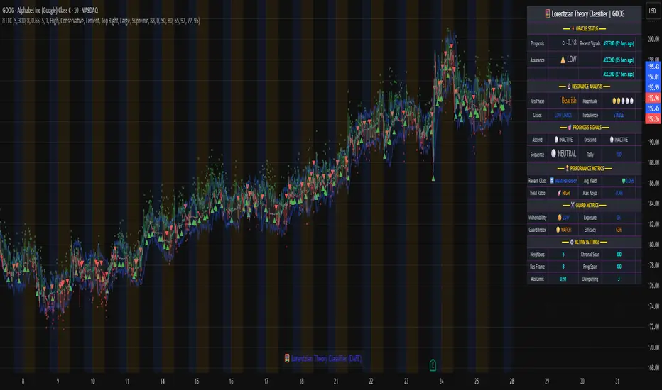
The dashboard is not a data table; it is your command interface with market reality. It translates the intricate dance of probabilities and vectors into clear, actionable intelligence.
⚡ ORACLE STATUS
Prognosis: The primary directional vector. Its color, magnitude, and emoji (⚡) reveal the strength and conviction of the Oracle's forward guidance.
Assurance: A real-time gauge of prediction quality, from "LOW" (high uncertainty) to "ELITE" (overwhelming statistical consensus). Interpret this as your core risk metric: trade with conviction when Assurance is ELITE; trade with caution when it is LOW.
🔮 RESONANCE ANALYSIS
Chaos: A direct measurement of market entropy. "LOW CHAOS" signifies a predictable, orderly regime. "HIGH CHAOS" is a warning of randomness and unpredictability, where trend-following logic may fail.
Turbulence: A measure of raw volatility. When the market is "TURBULENT," expect wider price swings and increased risk. Use this metric to adjust stop-loss distances and profit targets dynamically.
🏆 PERFORMANCE & ⚔️ GUARD METRICS
These sections provide illustrative statistics on the script's recent historical behavior. Metrics like Yield Ratio and Guard Index offer a quick heuristic on the prevailing risk-reward environment. Crucially, these are for observational context only and are not a substitute for your own rigorous testing and analysis.
🎨 THE VISUAL MANIFESTATION: Charting the Unseen
The LTC's visuals are designed to transform your chart from a 2D price graph into a 4D informational battlespace.
The Dynamic Aura (Background Color): This is the ambient energy field of the market. A luminous green (Ascend) signifies a bullish resonance field; a deep red (Descend) indicates bearish pressure.
The Assurance Shroud (Blue Bands): A visualization of confidence. When the shroud is wide and expansive , the Oracle's vision is clear and its predictions are robust.
The Prognosis Arc (Curved Line): A geodesic projection of the market's most likely path, based on the current Prognosis.
The Turbulence Cloud (Orange Mist): A visual warning system for market chaos. When this entropic mist expands , it is a clear sign that you are navigating a nebula of high unpredictability.
Oracle Markers (▲▼): The final, validated signals. These are not merely pivot points. They are moments in spacetime where a structural pivot has been confirmed and then ratified by a high-conviction vote from the Lorentzian Oracle. They are the pinnacles of confluence.
The Analyst's Observatory: The LTC transforms your chart into a command center for market analysis, providing a complete, at-a-glance view of market state, risk, and probabilistic trajectory.
🔧 THE ARCHITECT'S VISION: From a Blank Slate to a New Cosmos
The LTC was not assembled; it was derived. It began not with code, but with first principles, asking: "If we were to build an instrument to measure the market today, unbound by the technical dogmas of the 20th century, what would it look like?" The answer was clear: it must be multi-dimensional, it must be adaptive, and it must be built on a mathematical framework that respects the "fat-tailed" nature of reality.
The decision to use a pure Lorentzian kernel was non-negotiable. It represented a commitment to intellectual honesty over computational ease. The development of the Supreme Dashboard was driven by the philosophy of the "glass cockpit"—a belief that a trader's greatest asset is not a black box signal, but a transparent and intuitive flow of high-quality information. This script is the result of that unwavering vision: to create not just another indicator, but a new lens through which to perceive the market.
⚠️ RISK DISCLOSURE & PHILOSOPHY OF USE
The Lorentzian Theory Classifier is an instrument of profound analytical power, intended for the serious, discerning trader. It does not generate infallible signals. It generates high-probability, data-driven hypotheses based on a rigorous and transparent methodology. All trading involves substantial risk, and the future is fundamentally unknowable. Past performance, whether real or simulated, is no guarantee of future results. Use this tool to augment your own skill, to confirm your own analysis, and to manage your own risk within a well-defined trading plan.
"The effort to understand the universe is one of the very few things that lifts human life a little above the level of farce, and gives it some of the grace of tragedy."
— Steven Weinberg, Nobel Laureate in Physics
Trade with rigor. Trade with perspective. Trade with enlightenment. Trade with insight. Trade with anticipation.
— Dskyz, for DAFE Trading Systems
[Pandora] Laguerre Ultimate Explorations MulticatorIt's time to begin demonstrations differentiating the difference between known and actual feasibility beyond imagination... Welcome to my algorithmic twilight zone .
INTRODUCTION:
Hot off my press, I present this Laguerre multicator employing PSv6.0, originally formulated by John Ehlers for TASC - July 2025 Traders Tips. Basically I transcended Ehlers' notions of transversal filtration with an overhaul of his Laguerre design with my "what if" Pandora notions included. Striving beyond John Ehlers' original intended design. This action packed indicator is a radically revamped version of his original filter using novel techniques. My aim was to explore whether providing even more enhanced responsiveness and lesser lag is possible and how. Presented here is my mind warping results to witness.
EHLERS' LAGUERRE EXPLAINED:
First and foremost, the concept of Ehlers' Laguerre-izing method deserves a comprehensive deep dive. Ehlers' Laguerre filter design, as it functions originally, begins with his Ultimate Smoother (US) followed by a gang of four LERP (jargon for Linear intERPolation) filters. Following a myriad of cascading LERPs is a window-like FIR filter tapped into the LERP delay values to provide extra smoothness via the output.
On a side note, damping factor controlled LERP filters resemble EMAs indeed, but aren't exactly "periodic" filters that would have a period/length parameter and their subsequent calculations. I won't go into fine-grained relationship details, but EMA and LERP are indeed related in approach, being cousins of similar pedigree.
EXAMINING LAGUERRE:
I focused firstly on US initialization obstacles at Pine's bar_index==0 with nz() in abundance. The next primary notion of intrigue I mostly wondered about was, why are there four LERP elements instead of fewer or more. Why not three or why not two LERPs, etc... 1-4-6-4-1, I remember seeing those coefficients before in high pass filters.
Gathering my thoughts from that highpass knowledge base, I devised other tapped configuration modes to inspect their behavior out of curiosity. Eureka! There is actually more to Laguerre than Ehlers' mind provided, now that I had formulated additional modes. Each mode exhibits it's own lag/smoothness characteristics better than the quad LERPed version. I narrowed it down to a total of 5 modes for exploration. Mode 0 is just the raw US by itself.
ANALYZING FILTER BEHAVIORS:
Which option might be possibly superior, and how may I determine that? Fortunately, I have a custom-built analyzer allowing me to thoroughly examine transient responses across multiple periodicities simultaneously, providing remarkable visual insights.
While Ehlers has meagerly touched upon presenting general frequency responses in his books, I have excelled far beyond that. This robust filter analysis capability enables me to observe finer aspects hidden to others, ultimately leading to the deprecation of numerous existing filters. Not only this, but inventing entirely new species of filtration whether lowpass, highpass, or bandpass is already possible with a thorough comprehensive evaluation.
Revealing what's quirky with each filter and having the ability to discover what filters may be lacking in performance, is one of it's implications. I'm just going to explain this: For example US has a little too much overshoot to my liking, along with nonconformant cutoff frequency compliance with the period parameter. Perhaps Ehlers should inspect US coefficients a bit closer... I hope stating this is not received in an ill manner, as it's not my intention here.
What this technically eludes to is that UltimateSmoother can be further improved, analogous to my Laguerre alterations described above. I will also state Laguerre can indeed be reformulated to an even greater extent concerning group delay, from what I have already discussed. Another exciting time though... More investigative research is warranted.
LAGUERRE CONCLUSIONS:
After analyzing Laguerre's frequency compliance, transient responses, amplitudes, lag, symmetry across periodicities, noise rejection, and smoothness... I favor mode 3 for a multitude of reasons over the mode 4 configuration, but mostly superb smoothing with less lag, AND I also appreciated mode 1 & 2 for it's lower lag performance options.
Each mode and lag (phase shift) damping value has it's own unique characteristics at extremes, yet they demonstrate additional finesse in it's new hybrid form without adding too much more complexity. This multicator has a bunch of Laguerre filters in the overlay chart over many periodicities so you can easily witness it's differing periodic symmetries on an input signal while adjusting lag and mode.
LAGUERRE OSCILLATOR:
The oscillator is integrated into the laguerreMulti() function for the intention of posterity only. I performed no evaluation on it, only providing the code in Pine. That wasn't part of my intended exploration adventure, as I'm more TREND oriented for the time being, focusing my efforts there.
Market analysis has two primary aspects in my observations, one cyclic while the other is trending dynamics... There's endless oscillators, but my expectations for trend analysis seems a little lesser explored in my opinion, hence my laborious trend endeavors. Ehlers provided both indicator facets this time around, and I hope you find the filtration aspect more intriguing after absorption of this reading.
FUNCTION MODULES EXPLAINED:
The Ultimate Smoother is an advanced IIR lowpass smoothing filter intended to minimize noise in time series data with minimal group delay, similar to a traditional biquad filter. This calculation helps to create a smoother version of the original signal without the distortions of short-term fluctuations and with minimal lag, adjustable by period.
The Modified Laguerre Lowpass Filter (MLLF) enhances the functionality of US by introducing a Laguerre mode parameter along side the lag parameter to refine control over the amount of additional smoothing/lag applied to the signal. By tethering US with this LERPed lag mechanism, MLLF achieves an effective balance between responsiveness and smoothness, allowing for customizable lag adjustments via multiple inputs. This filter ends with selecting from a choice of weighted averages derived from a gang of up to four cascading LERP calculations, resulting with smoother representations of the data.
The Laguerre Oscillator is a momentum-like indicator derived from the output of US and a singular LERPed lowpass filter. It calculates the difference between the US data and Laguerre filter data, normalizing it by the root mean square (RMS). This quasi-normalization technique helps to assess the intensity of the momentum on any timeframe within an expected bound range centered around 0.0. When the Laguerre Oscillator is positive, it suggests that the smoothed data is trending upward, while a negative value indicates a downward trend. Adjustability is controlled with period, lag, Laguerre mode, and RMS period.

Reversal Point Dynamics⇋ Reversal Point Dynamics (RPD)
This is not an indicator; it is a complete system for deconstructing the mechanics of a market reversal. Reversal Point Dynamics (RPD) moves far beyond simplistic pattern recognition, venturing into a deep analysis of the underlying forces that cause trends to exhaust, pause, and turn. It is engineered from the ground up to identify high-probability reversal points by quantifying the confluence of market dynamics in real-time.
Where other tools provide a static signal, RPD delivers a dynamic probability. It understands that a true market turning point is not a single event, but a cascade of failing momentum, structural breakdown, and a shift in market order. RPD's core engine meticulously analyzes each of these dynamic components—the market's underlying state, its velocity and acceleration, its degree of chaos (entropy), and its structural framework. These forces are synthesized into a single, unified Probability Score, offering you an unprecedented, transparent view into the conviction behind every potential reversal.
This is not a "black box" system. It is an open-architecture engine designed to empower the discerning trader. Featuring real-time signal projection, an integrated Fibonacci R2R Target Engine, and a comprehensive dashboard that acts as your Dynamics Control Center , RPD gives you a complete, holistic view of the market's state.
The Theoretical Core: Deconstructing Market Dynamics
RPD's analytical power is born from the intelligent synthesis of multiple, distinct theoretical models. Each pillar of the engine analyzes a different facet of market behavior. The convergence of these analyses—the "Singularity" event referenced in the dashboard—is what generates the final, high-conviction probability score.
1. Pillar One: Quantum State Analysis (QSA)
This is the foundational analysis of the market's current state within its recent context. Instead of treating price as a random walk, QSA quantizes it into a finite number of discrete "states."
Formulaic Concept: The engine establishes a price range using the highest high and lowest low over the Adaptive Analysis Period. This range is then divided into a user-defined number of Analysis Levels. The current price is mapped to one of these states (e.g., in a 9-level system, State 0 is the absolute low, and State 8 is the absolute high).
Analytical Edge: This acts as a powerful foundational filter. The engine will only begin searching for reversal signals when the market has reached a statistically stretched, extreme state (e.g., State 0 or 8). The Edge Sensitivity input allows you to control exactly how close to this extreme edge the price must be, ensuring you are trading from points of maximum potential exhaustion.
2. Pillar Two: Price State Roc (PSR) - The Dynamics of Momentum
This pillar analyzes the kinetic forces of the market: its velocity and acceleration. It understands that it’s not just where the price is, but how it got there that matters.
Formulaic Concept: The psr function calculates two derivatives of price.
Velocity: (price - price ). This measures the speed and direction of the current move.
Acceleration: (velocity - velocity ). This measures the rate of change in that speed. A negative acceleration (deceleration) during a strong rally is a critical pre-reversal warning, indicating momentum is fading even as price may be pushing higher.
Analytical Edge: The engine specifically hunts for exhaustion patterns where momentum is clearly decelerating as price reaches an extreme state. This is the mechanical signature of a weakening trend.
3. Pillar Three: Market Entropy Analysis - The Dynamics of Order & Chaos
This is RPD's chaos filter, a concept borrowed from information theory. Entropy measures the degree of randomness or disorder in the market's price action.
Formulaic Concept: The calculateEntropy function analyzes recent price changes. A market moving directionally and smoothly has low entropy (high order). A market chopping back and forth without direction has high entropy (high chaos). The value is normalized between 0 and 1.
Analytical Edge: The most reliable trades occur in low-entropy, ordered environments. RPD uses the Entropy Threshold to disqualify signals that attempt to form in chaotic, unpredictable conditions, providing a powerful shield against whipsaw markets.
4. Pillar Four: The Synthesis Engine & Probability Calculation
This is where all the dynamic forces converge. The final probability score is a weighted calculation that heavily rewards confluence.
Formulaic Concept: The calculateProbability function intelligently assembles the final score:
A Base Score is established from trend strength and entropy.
An Entropy Score adds points for low entropy (order) and subtracts for high entropy (chaos).
A significant Divergence Bonus is awarded for a classic momentum divergence.
RSI & Volume Bonuses are added if momentum oscillators are in extreme territory or a volume spike confirms institutional interest.
MTF & Adaptive Bonuses add further weight for alignment with higher timeframe structure.
Analytical Edge: A signal backed by multiple dynamic forces (e.g., extreme state + decelerating momentum + low entropy + volume spike) will receive an exponentially higher probability score. This is the very essence of analyzing reversal point dynamics.
The Command Center: Mastering the Inputs
Every input is a precise lever of control, allowing you to fine-tune the RPD engine to your exact trading style, market, and timeframe.
🧠 Core Algorithm
Predictive Mode (Early Detection):
What It Is: Enables the engine to search for potential reversals on the current, unclosed bar.
How It Works: Analyzes intra-bar acceleration and state to identify developing exhaustion. These signals are marked with a ' ? ' and are tentative.
How To Use It: Enable for scalping or very aggressive day trading to get the earliest possible indication. Disable for swing trading or a more conservative approach that waits for full bar confirmation.
Live Signal Mode (Current Bar):
What It Is: A highly aggressive mode that plots tentative signals with a ' ! ' on the live bar based on projected price and momentum. These signals repaint intra-bar.
How It Works: Uses a linear regression projection of the close to anticipate a reversal.
How To Use It: For advanced users who use intra-bar dynamics for execution and understand the nature of repainting signals.
Adaptive Analysis Period:
What It Is: The main lookback period for the QSA, PSR, and Entropy calculations. This is the engine's "memory."
How It Works: A shorter period makes the engine highly sensitive to local price swings. A longer period makes it focus only on major, significant market structure.
How To Use It: Scalping (1-5m): 15-25. Day Trading (15m-1H): 25-40. Swing Trading (4H+): 40-60.
Fractal Strength (Bars):
What It Is: Defines the strength of the pivot detection used for confirming reversal events.
How It Works: A value of '2' requires a candle's high/low to be more extreme than the two bars to its left and right.
How To Use It: '2' is a robust standard. Increase to '3' for an even stricter definition of a structural pivot, which will result in fewer signals.
MTF Multiplier:
What It Is: Integrates pivot data from a higher timeframe for confluence.
How It Works: A multiplier of '4' on a 15-minute chart will pull pivot data from the 1-hour chart (15 * 4 = 60m).
How To Use It: Set to a multiple that corresponds to your preferred higher timeframe for contextual analysis.
🎯 Signal Settings
Min Probability %:
What It Is: Your master quality filter. A signal is only plotted if its score exceeds this threshold.
How It Works: Directly filters the output of the final probability calculation.
How To Use It: High-Quality (80-95): For A+ setups only. Balanced (65-75): For day trading. Aggressive (50-60): For scalping.
Min Signal Distance (Bars):
What It Is: A noise filter that prevents signals from clustering in choppy conditions.
How It Works: Enforces a "cooldown" period of N bars after a signal.
How To Use It: Increase in ranging markets to focus on major swings. Decrease on lower timeframes.
Entropy Threshold:
What It Is: Your "chaos shield." Sets the maximum allowable market randomness for a signal.
How It Works: If calculated entropy is above this value, the signal is invalidated.
How To Use It: Lower values (0.1-0.5): Extremely strict. Higher values (0.7-1.0): More lenient. 0.85 is a good balance.
Adaptive Entropy & Aggressive Mode:
What It Is: Toggles for dynamically adjusting the engine's core parameters.
How It Works: Adaptive Entropy can slightly lower the required probability in strong trends. Aggressive Mode uses more lenient settings across the board.
How To Use It: Keep Adaptive on. Use Aggressive Mode sparingly, primarily for scalping highly volatile assets.
📊 State Analysis
Analysis Levels:
What It Is: The number of discrete "states" for the QSA.
How It Works: More levels create a finer-grained analysis of price location.
How To Use It: 6-7 levels are ideal. Increasing to 9 can provide more precision on very volatile assets.
Edge Sensitivity:
What It Is: Defines how close to the absolute top/bottom of the range price must be.
How It Works: '0' means price must be in the absolute highest/lowest state. '3' allows a signal within the top/bottom 3 states.
How To Use It: '3' provides a good balance. Lower it to '1' or '0' if you only want to trade extreme exhaustion.
The Dashboard: Your Dynamics Control Center
The dashboard provides a transparent, real-time view into the engine's brain. Use it to understand the context behind every signal and to gauge the current market environment at a glance.
🎯 UNIFIED PROB SCORE
TOTAL SCORE: The highest probability score (either Peak or Valley) the engine is currently calculating. This is your main at-a-glance conviction metric. The "Singularity" header refers to the event where market dynamics align—the event RPD is built to detect.
Quality: A human-readable interpretation of the Total Score. "EXCEPTIONAL" (🌟) is a rare, A+ confluence event. "STRONG" (💪) is a high-quality, tradable setup.
📊 ORDER FLOW & COMPONENT ANALYSIS
Volume Spike: Shows if the current volume is significantly higher than average (YES/NO). A 'YES' adds major confirmation.
Peak/Valley Conf: This breaks down the probability score into its directional components, showing you the separate confidence levels for a potential top (Peak) versus a bottom (Valley).
🌌 MARKET STRUCTURE
HTF Trend: Shows the direction of the underlying trend based on a Supertrend calculation.
Entropy: The current market chaos reading. "🔥 LOW" is an ideal, ordered state for trading. "😴 HIGH" is a warning of choppy, unpredictable conditions.
🔮 FIB & R2R ZONE (Large Dashboard)
This section gives you the status of the Fibonacci Target Engine. It shows if an Active Channel (entry zone) or Stop Zone (invalidation zone) is active and displays the precise price levels for the static entry, target, and stop calculated at the time of the signal.
🛡️ FILTERS & PREDICTIVES (Large Dashboard)
This panel provides a status check on all the bonus filters. It shows the current RSI Status, whether a Divergence is present, and if a Live Pending signal is forming.
The Visual Interface: A Symphony of Data
Every visual element is designed for instant, intuitive interpretation of market dynamics.
Signal Markers: These are the primary outputs of the engine.
▼/▲ b: A fully confirmed signal that has passed all filters.
? b: A tentative signal generated in Predictive Mode, indicating developing dynamics.
◈ b: This diamond icon replaces the standard triangle when the signal is confirmed by a strong momentum divergence, highlighting it as a superior setup where dynamics are misaligned with price.
Harmonic Wave: The flowing, colored wave around the price.
What It Represents: The market's "flow dynamic" and volatility.
How to Interpret It: Expanding waves show increasing volatility. The color is tied to the "Quantum Color" in your theme, representing the underlying energy field of the market.
Entropy Particles: The small dots appearing above/below price.
What They Represent: A direct visualization of the "order dynamic."
How to Interpret Them: Their presence signifies a low-entropy, ordered state ideal for trading. Their color indicates the direction of momentum (PSR velocity). Their absence means the market is too chaotic (high entropy).
The Fibonacci Target Engine: The dynamic R2R system appearing post-signal.
Static Fib Levels: Colored horizontal lines representing the market's "structural dynamic."
The Green "Active Channel" Box: Your zone of consideration. An area to manage a potential entry.
Development Philosophy
Reversal Point Dynamics was engineered to answer a fundamental question: can we objectively measure the forces behind a market turn? It is a synthesis of concepts from market microstructure, statistics, and information theory. The objective was never to create a "perfect" system, but to build a robust decision-support tool that provides a measurable, statistical edge by focusing on the principle of confluence.
By demanding that multiple, independent market dynamics align simultaneously, RPD filters out the vast majority of market noise. It is designed for the trader who thinks in terms of probability and risk management, not in terms of certainties. It is a tool to help you discount the obvious and bet on the unexpected alignment of market forces.
"Markets are constantly in a state of uncertainty and flux and money is made by discounting the obvious and betting on the unexpected."
— George Soros
Trade with insight. Trade with anticipation.
— Dskyz, for DAFE Trading Systems

Gold vs DXYThe 30-day rolling correlation between Gold (XAU/USD) and the US Dollar Index (DXY) shows how closely the two move together — or more often, in opposite directions — over the last 30 trading days. In most market environments, the relationship is pretty straightforward: when the dollar goes up, gold tends to go down, and vice versa. That’s because gold is priced in dollars, so a stronger dollar makes it more expensive for international buyers, which usually softens demand.
But it’s not always that simple. There are times when this inverse correlation breaks down. For example, if real yields (like the US 10-year yield minus inflation expectations) are rising, that can pressure gold even if the dollar is falling — because higher real returns elsewhere make gold less attractive. Another case is when other currencies, like the euro or yen, rally strongly on their own central bank decisions. This can pull DXY lower without necessarily signaling weakness in the U.S. economy — meaning gold might not benefit much.
There are also “risk-on” moments where investors rotate into equities or crypto, selling off both gold and the dollar in favor of yield or momentum. And during periods of crisis or uncertainty, both gold and the dollar can rise together as safe-haven assets, breaking the usual pattern entirely.
That’s why tracking the rolling correlation is helpful. It shows whether the historical relationship between gold and the dollar is still holding — or if we’re entering a different market regime. It’s not about predicting exact price moves, but about understanding the current backdrop. When gold and DXY are moving out of sync as expected, it can support your trade thesis. But when the correlation flattens or flips, it’s often a sign to dig deeper — macro forces may be shifting.

🌊 Reinhart-Rogoff Financial Instability Index (RR-FII)Overview
The Reinhart-Rogoff Financial Instability Index (RR-FII) is a multi-factor indicator that consolidates historical crisis patterns into a single risk score ranging from 0 to 100. Drawing from the extensive research in "This Time is Different: Eight Centuries of Financial Crises" by Carmen M. Reinhart and Kenneth S. Rogoff, the RR-FII translates nearly a millennium of crisis data into practical insights for financial markets.
What It Does
The RR-FII acts like a real-time financial weather forecast by tracking four key stress indicators that historically signal the build-up to major financial crises. Unlike traditional indicators based only on price, it takes a broader view, examining the global market's interconnected conditions to provide a holistic assessment of systemic risk.
The Four Crisis Components
- Capital Flow Stress (Default weight: 25%)
- Data analyzed: Volatility (ATR) and price movements of the selected asset.
- Detects abrupt volatility surges or sharp price falls, which often precede debt defaults due to sudden stops in capital inflow.
- Commodity Cycle (Default weight: 20%)
- Data analyzed: US crude oil prices (customizable).
- Watches for significant declines from recent highs, since commodity price troughs often signal looming crises in emerging markets.
- Currency Crisis (Default weight: 30%)
- Data analyzed: US Dollar Index (DXY, customizable).
- Flags if the currency depreciates by more than 15% in a year, aligning with historical criteria for currency crashes linked to defaults.
- Banking Sector Health (Default weight: 25%)
- Data analyzed: Performance of financial sector ETFs (e.g., XLF) relative to broad market benchmarks (SPY).
- Monitors for underperformance in the financial sector, a strong indicator of broader financial instability.
Risk Scale Interpretation
- 0-20: Safe – Low systemic risk, normal conditions.
- 20-40: Moderate – Some signs of stress, increased caution advised.
- 40-60: Elevated – Multiple risk factors, consider adjusting positions.
- 60-80: High – Significant probability of crisis, implement strong risk controls.
- 80-100: Critical – Several crisis indicators active, exercise maximum caution.
Visual Features
- The main risk line changes color with increasing risk.
- Background colors show different risk zones for quick reference.
- Option to view individual component scores.
- A real-time status table summarizes all component readings.
- Crisis event markers appear when thresholds are breached.
- Customizable alerts notify users of changing risk levels.
How to Use
- Apply as an overlay for broad risk management at the portfolio level.
- Adjust position sizes inversely to the crisis index score.
- Use high index readings as a warning to increase vigilance or reduce exposure.
- Set up alerts for changes in risk levels.
- Analyze using various timeframes; daily and weekly charts yield the best macro insights.
Customizable Settings
- Change the weighting of each crisis factor.
- Switch commodity, currency, banking sector, and benchmark symbols for customized views or regional focus.
- Adjust thresholds and visual settings to match individual risk preferences.
Academic Foundation
Rooted in rigorous analysis of 66 countries and 800 years of data, the RR-FII uses empirically validated relationships and thresholds to assess systemic risk. The indicator embodies key findings: financial crises often follow established patterns, different types of crises frequently coincide, and clear quantitative signals often precede major events.
Best Practices
- Use RR-FII as part of a comprehensive risk management strategy, not as a standalone trading signal.
- Combine with fundamental analysis for complete market insight.
- Monitor for differences between component readings and the overall index.
- Favor higher timeframes for a broader macro view.
- Adjust component importance to suit specific market interests.
Important Disclaimers
- RR-FII assesses risk using patterns from past crises but does not predict future events.
- Historical performance is not a guarantee of future results.
- Always employ proper risk management.
- Consider this tool as one element in a broader analytical toolkit.
- Even with high risk readings, markets may not react immediately.
Technical Requirements
- Compatible with Pine Script v6, suitable for all timeframes and symbols.
- Pulls data automatically for USOIL, DXY, XLF, and SPY.
- Operates without repainting, using only confirmed data.
The RR-FII condenses centuries of financial crisis knowledge into a modern risk management tool, equipping investors and traders with a deeper understanding of when systemic risks are most pronounced.

Fibonacci Sequence Moving Average [BackQuant]Fibonacci Sequence Moving Average with Adaptive Oscillator
1. Overview
The Fibonacci Sequence Moving Average indicator is a two‑part trading framework that combines a custom moving average built from the famous Fibonacci number set with a fully featured oscillator, normalisation engine and divergence suite. The moving average half delivers an adaptive trend line that respects natural market rhythms, while the oscillator half translates that trend information into a bounded momentum stream that is easy to read, easy to compare across assets and rich in confluence signals. Everything from weighting logic to colour palettes can be customised, so the tool comfortably fits scalpers zooming into one‑minute candles as well as position traders running multi‑month trend following campaigns.
2. Core Calculation
Fibonacci periods – The default length array is 5, 8, 13, 21, 34. A single multiplier input lets you scale the whole family up or down without breaking the golden‑ratio spacing. For example a multiplier of 3 yields 15, 24, 39, 63, 102.
Component averages – Each period is passed through Simple Moving Average logic to produce five baseline curves (ma1 through ma5).
Weighting methods – You decide how those five values are blended:
• Equal weighting treats every curve the same.
• Linear weighting applies factors 1‑to‑5 so the slowest curve counts five times as much as the fastest.
• Exponential weighting doubles each step for a fast‑reacting yet still smooth line.
• Fibonacci weighting multiplies each curve by its own period value, honouring the spirit of ratio mathematics.
Smoothing engine – The blended average is then smoothed a second time with your choice of SMA, EMA, DEMA, TEMA, RMA, WMA or HMA. A short smoothing length keeps the result lively, while longer lengths create institution‑grade glide paths that act like dynamic support and resistance.
3. Oscillator Construction
Once the smoothed Fib MA is in place, the script generates a raw oscillator value in one of three flavours:
• Distance – Percentage distance between price and the average. Great for mean‑reversion.
• Momentum – Percentage change of the average itself. Ideal for trend acceleration studies.
• Relative – Distance divided by Average True Range for volatility‑aware scaling.
That raw series is pushed through a look‑back normaliser that rescales every reading into a fixed −100 to +100 window. The normalisation window defaults to 100 bars but can be tightened for fast markets or expanded to capture long regimes.
4. Visual Layer
The oscillator line is gradient‑coloured from deep red through sky blue into bright green, so you can spot subtle momentum shifts with peripheral vision alone. There are four horizontal guide lines: Extreme Bear at −50, Bear Threshold at −20, Bull Threshold at +20 and Extreme Bull at +50. Soft fills above and below the thresholds reinforce the zones without cluttering the chart.
The smoothed Fib MA can be plotted directly on price for immediate trend context, and each of the five component averages can be revealed for educational or research purposes. Optional bar‑painting mirrors oscillator polarity, tinting candles green when momentum is bullish and red when momentum is bearish.
5. Divergence Detection
The script automatically looks for four classes of divergences between price pivots and oscillator pivots:
Regular Bullish, signalling a possible bottom when price prints a lower low but the oscillator prints a higher low.
Hidden Bullish, often a trend‑continuation cue when price makes a higher low while the oscillator slips to a lower low.
Regular Bearish, marking potential tops when price carves a higher high yet the oscillator steps down.
Hidden Bearish, hinting at ongoing downside when price posts a lower high while the oscillator pushes to a higher high.
Each event is tagged with an ℝ or ℍ label at the oscillator pivot, colour‑coded for clarity. Look‑back distances for left and right pivots are fully adjustable so you can fine‑tune sensitivity.
6. Alerts
Five ready‑to‑use alert conditions are included:
• Bullish when the oscillator crosses above +20.
• Bearish when it crosses below −20.
• Extreme Bullish when it pops above +50.
• Extreme Bearish when it dives below −50.
• Zero Cross for momentum inflection.
Attach any of these to TradingView notifications and stay updated without staring at charts.
7. Practical Applications
Swing trading trend filter – Plot the smoothed Fib MA on daily candles and only trade in its direction. Enter on oscillator retracements to the 0 line.
Intraday reversal scouting – On short‑term charts let Distance mode highlight overshoots beyond ±40, then fade those moves back to mean.
Volatility breakout timing – Use Relative mode during earnings season or crypto news cycles to spot momentum surges that adjust for changing ATR.
Divergence confirmation – Layer the oscillator beneath price structure to validate double bottoms, double tops and head‑and‑shoulders patterns.
8. Input Summary
• Source, Fibonacci multiplier, weighting method, smoothing length and type
• Oscillator calculation mode and normalisation look‑back
• Divergence look‑back settings and signal length
• Show or hide options for every visual element
• Full colour and line width customisation
9. Best Practices
Avoid using tiny multipliers on illiquid assets where the shortest Fibonacci window may drop under three bars. In strong trends reduce divergence sensitivity or you may see false counter‑trend flags. For portfolio scanning set oscillator to Momentum mode, hide thresholds and colour bars only, which turns the indicator into a heat‑map that quickly highlights leaders and laggards.
10. Final Notes
The Fibonacci Sequence Moving Average indicator seeks to fuse the mathematical elegance of the golden ratio with modern signal‑processing techniques. It is not a standalone trading system, rather a multi‑purpose information layer that shines when combined with market structure, volume analysis and disciplined risk management. Always test parameters on historical data, be mindful of slippage and remember that past performance is never a guarantee of future results. Trade wisely and enjoy the harmony of Fibonacci mathematics in your technical toolkit.

Weighted Multi-Mode Oscillator [BackQuant]Weighted Multi‑Mode Oscillator
1. What Is It?
The Weighted Multi‑Mode Oscillator (WMMO) is a next‑generation momentum tool that turns a dynamically‑weighted moving average into a 0‑100 bounded oscillator.
It lets you decide how each bar is weighted (by volume, volatility, momentum or a hybrid blend) and how the result is normalised (Percentile, Z‑Score or Min‑Max).
The outcome is a self‑adapting gauge that delivers crystal‑clear overbought / oversold zones, divergence clues and regime shifts on any market or timeframe.
2. How It Works
• Dynamic Weight Engine
▪ Volume – emphasises bars with exceptional participation.
▪ Volatility – inverse ATR weighting filters noisy spikes.
▪ Momentum – amplifies strong directional ROC bursts.
▪ Hybrid – equal‑weight blend of the three dimensions.
• Multi‑Mode Smoothing
Choose from 8 MA types (EMA, DEMA, HMA, LINREG, TEMA, RMA, SMA, WMA) plus a secondary smoothing factor to fine‑tune lag vs. responsiveness.
• Normalization Suite
▪ Percentile – rank vs. recent history (context aware).
▪ Z‑Score – standard deviations from mean (statistical extremes).
▪ Min‑Max – scale between rolling high/low (trend friendly).
3. Reading the Oscillator
Zone Default Level Interpretation
Bull > 80 Acceleration; momentum buyers in control
Neutral 20 – 80 Consolidation / no edge
Bear < 20 Exhaustion; sellers dominate
Gradient line/area automatically shades from bright green (strong bull) to deep red (strong bear).
Optional bar‑painting colours price bars the same way for rapid chart scanning.
4. Typical Use‑Cases
Trend Confirmation – Set Weight = Hybrid, Smoothing = EMA. Enter pullbacks only when WMMO > 50 and rising.
Mean Reversion – Weight = Volatility, reduce upper / lower bands to 70 / 30 and fade extremes.
Volume Pulse – Intraday futures: Weight = Volume to catch participation surges before breakout candles.
Divergence Spotting – Compare price highs/lows to WMMO peaks for early reversal clues.
5. Inputs & Styling
Calculation: Source, MA Length, MA Type, Smoothing
Weighting: Volume period & factor, Volatility length, Momentum period
Normalisation: Method, Look‑back, Upper / Lower thresholds
Display: Gradient fills, Threshold lines, Bar‑colouring toggle, Line width & colours
All thresholds, colours and fills are fully customisable inside the settings panel.
6. Built‑In Alerts
WMMO Long – oscillator crosses up through upper threshold.
WMMO Short – oscillator crosses down through lower threshold.
Attach them once and receive push / e‑mail notifications the moment momentum flips.
7. Best Practices
Percentile mode is self‑adaptive and works well across assets; Z‑Score excels in ranges; Min‑Max shines in persistent trends.
Very short MA lengths (< 10) may produce jitter; compensate with higher “Smoothing” or longer look‑backs.
Pair WMMO with structure‑based tools (S/R, trend lines) for higher‑probability trade confluence.
Disclaimer
This script is provided for educational purposes only. It is not financial advice. Always back‑test thoroughly and manage risk before trading live capital.

Multi Pivot Point & Central Pivot Range - Nadeem Al-QahwiThis indicator combines four advanced trading modules into one flexible and easy-to-use script:
Traditional Pivot Points:
Calculates classic support and resistance levels (PP, R1–R5, S1–S5) based on previous session data. Ideal for identifying key turning points and mapping out the daily, weekly, or monthly structure.
Camarilla Levels:
Provides six upper and lower pivot levels (H1–H6, L1–L6) derived from volatility and closing price formulas. Especially effective for intraday reversal, mean reversion, and finding overbought/oversold extremes.
Central Pivot Range (CPR):
Plots the median, top, and bottom of the value area each session. CPR width instantly highlights whether the market is likely to trend (narrow CPR) or remain range-bound (wide CPR).
Developing CPR projects the evolving range for the current period—essential for real-time analysis and pre-market planning.
Dynamic Zone Levels (DZL):
Automatically detects and highlights clusters of pivots to reveal high-probability support/resistance zones, filtering out market “noise.”
DZL alerts notify you whenever price breaks or retests these key areas, making it easier to spot momentum trades and avoid false signals.
Key Features:
Multi-timeframe flexibility: Use with daily, weekly, monthly, yearly, or custom timeframes—even rare ones like biyearly and decennial.
Modular design: Activate or hide any system (Traditional, Camarilla, CPR, DZL) as you need.
Bilingual interface: Every setting and label is shown in both English and Arabic.
Full customization: Control visibility, color, style, and placement for every level and label.
Historical depth: Plot up to 5,000 pivot/zones back for deep analysis and backtesting.
Smart alerts: Get instant notifications on true S/R breakouts or retests (from DZL).
How to Use:
Trend Trading:
Watch for a very narrow CPR to identify potential trending days—trade in the breakout direction above/below the CPR.
Range Trading:
When CPR is wide, expect sideways movement. Fade reversals at R1/S1 or within the CPR boundaries.
Breakouts:
Use DZL alerts to capture momentum as price breaks or retests dynamic support/resistance zones.
Multi-Timeframe Confluence:
Combine CPR and pivot levels from multiple timeframes for higher-probability entries and exits.
All calculations and logic are fully open.
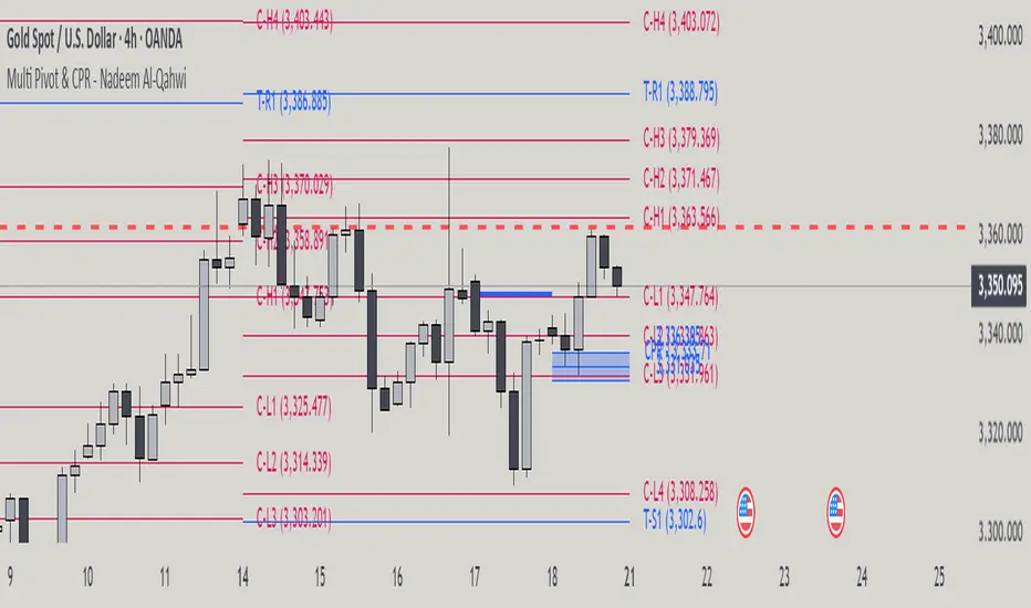
Ease of Movement Z-Score Trend | DextraGeneral Description:
The "Ease of Movement Z-Score Trend | Dextra" (EOM-Z Trend) is an innovative technical analysis tool that combines the Ease of Movement (EOM) concept with Z-Score to measure how easily price moves relative to volume, while identifying market trends with intuitive visualization. This indicator is designed to help traders detect uptrend and downtrend phases with precision, enhanced by candle coloring for direct trend representation on the chart.
Key Features
Ease of Movement (EOM): Measures how easily price moves based on the change in the midpoint price and volume, normalized with Z-Score for statistical analysis.
Z-Score Normalization: Provides an indication of deviations from the mean, enabling the identification of overbought or oversold conditions.
Adjustable Thresholds: Users can customize upper and lower thresholds to define trend boundaries.
Candle Coloring: Visual trend representation with green (uptrend), red (downtrend), and gray (neutral) candles.
Flexibility: Adjustable for different timeframes and assets.
How It Works
The indicator operates through the following steps:
EOM Calculation:
hl2 = (high + low) / 2: Calculates the average midpoint price per bar.
eom = ta.sma(10000 * ta.change(hl2) * (high - low) / volume, length): EOM is computed as the smoothed average of the price midpoint change multiplied by the price range per unit volume, scaled by 10,000, over length bars (default 20).
Z-Score Calculation:
mean_eom = ta.sma(eom, z_length): Average EOM over z_length bars (default 93).
std_dev_eom = ta.stdev(eom, z_length): Standard deviation of EOM.
z_score = (eom - mean_eom) / std_dev_eom: Z-Score indicating how far EOM deviates from its mean in standard deviation units.
Trend Detection:
upperthreshold (default 1.03) and lowerthreshold (default -1.63): Thresholds to classify uptrend (if Z-Score > upperthreshold) and downtrend (if Z-Score < lowerthreshold).
eom_is_up and eom_is_down: Logical variables for trend status.
Visualization:
plot(z_score, ...): Z-Score line plotted with green (uptrend), red (downtrend), or gray (neutral) coloring.
plotcandle(...): Candles colored green, red, or gray based on trend.
hline(...): Dashed lines marking the thresholds.
Input Settings
EOM Length (default 20): Period for calculating EOM, determining sensitivity to price changes.
Z-Score Lookback Period (default 93): Period for calculating the Z-Score mean and standard deviation.
Uptrend Threshold (default 1.03): Minimum Z-Score value to classify an uptrend.
Downtrend Threshold (default -1.93): Maximum Z-Score value to classify a downtrend.
How to Use
Installation: Add the indicator via the "Indicators" menu in TradingView and search for "EOM-Z Trend | Dextra".
Customization:
Adjust EOM Length and Z-Score Lookback Period based on the timeframe (e.g., 20 and 93 for daily timeframes).
Set Uptrend Threshold and Downtrend Threshold according to preference or asset characteristics (e.g., lower to 0.8 and -1.5 for volatile markets).
Interpretation:
Uptrend (Green): Z-Score above upperthreshold, indicating strong upward price movement.
Downtrend (Red): Z-Score below lowerthreshold, indicating significant downward movement.
Neutral (Gray): Conditions between thresholds, suggesting a sideways market.
Use candle coloring as the primary visual guide, combined with the Z-Score line for confirmation.
Advantages
Intuitive Visualization: Candle coloring simplifies trend identification without deep analysis.
Flexibility: Customizable parameters allow adaptation to various markets.
Statistical Analysis: Z-Score provides a robust perspective on price deviations from the norm.
No Repainting: The indicator uses historical data and does not alter values after a bar closes.
Limitations
Volume Dependency: Requires accurate volume data; an error occurs if volume is unavailable.
Market Context: Effectiveness depends on properly tuned thresholds for specific assets.
Lack of Additional Signals: No built-in alerts or supplementary confirmation indicators.
Recommendations
Ideal Timeframe: Daily (1D) or (2D) for stable trends.
Combination: Pair with others indicators for signal validation.
Optimization: Test thresholds on historical data of the traded asset for optimal results.
Important Notes
This indicator relies entirely on internal TradingView data (high, low, close, volume) and does not integrate on-chain data. Ensure your data provider supports volume to avoid errors. This version (1.0) is the initial release, with potential future updates including features like alerts or multi-timeframe analysis.
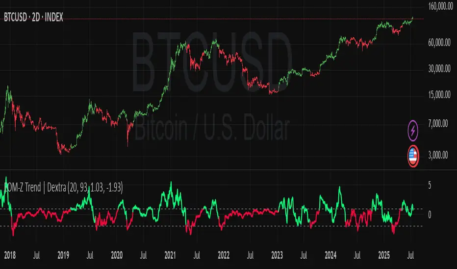
10/20 MA Coil: Progressive Colors & Multi-Day BreakoutThis indicator detects price “coil” setups and highlights potential breakout or breakdown opportunities using moving average alignment and volatility compression.
Features:
• Coil Detection:
• Identifies consolidation when:
• The 10 and 20 MAs are tightly aligned (within user-defined tolerance)
• Price is above both MAs and within 1.5x ADR of them
• The 50 MA is rising
• Progressive Coil Coloring:
• Coil candles are colored in progressively darker orange as the streak continues
• Bullish Breakout Signal:
• Triggers when a green candle follows a coiled bar
• The candle’s body must be greater than or equal to 1 ATR
• Colored lime green
• Bearish Breakdown Signal:
• Triggers when a red candle follows a coiled bar
• The candle’s body must be greater than or equal to 1 ATR to the downside
• Colored black
• Custom Candle Rendering:
• Candle body color represents coil or breakout state
• Wick and border are red or green to reflect price direction
• Optional Debug Tools:
• Coil streak, ATR, and distance from MAs can be plotted for deeper analysis
This script is designed for traders looking to spot price compression and prepare for high-probability moves following low-volatility setups.
Price Volume Trend [sgbpulse]1. Introduction: What is Price Volume Trend (PVT)?
The Price Volume Trend (PVT) indicator is a powerful technical analysis tool designed to measure buying and selling pressure in the market based on price changes relative to trading volume. Unlike other indicators that focus solely on volume or price, PVT combines both components to provide a more comprehensive picture of trend strength.
How is it Calculated?
The PVT is calculated by adding or subtracting a proportional part of the daily volume from a cumulative total.
When the closing price rises, a proportional part of the daily volume (based on the percentage price change) is added to the previous PVT value.
When the closing price falls, a proportional part of the daily volume is subtracted from the previous PVT value.
If there is no change in price, the PVT value remains unchanged.
The result of this calculation is a cumulative line that rises when buying pressure is strong and falls when selling pressure dominates.
2. Why PVT? Comparison to Similar Indicators
While other indicators measure volume-price pressure, PVT offers a unique advantage:
PVT vs. On-Balance Volume (OBV):
OBV simply adds or subtracts the entire day's volume based on the closing direction (up/down), regardless of the magnitude of the price change. This means a 0.1% price change is treated the same as a 10% change.
PVT, on the other hand, gives proportional weight to volume based on the percentage price change. A trading day with a large price increase and high volume will impact the PVT significantly more than a small price increase with the same volume. This makes PVT more sensitive to trend strength and changes within it.
PVT vs. Accumulation/Distribution Line (A/D Line):
The A/D Line focuses on the relationship between the closing price and the bar's trading range (Close Location Value) and multiplies it by volume. It indicates whether the pressure is buying or selling within a single bar.
PVT focuses on the change between closing prices of consecutive bars, multiplying this by volume. It better reflects the flow of money into or out of an asset over time.
By combining volume with percentage price change, PVT provides deeper insights into trend confirmation, identifying divergences between price and volume, and spotting signs of weakness or strength in the current trend.
3. Indicator Settings (Inputs)
The "Price Volume Trend " indicator offers great flexibility for customization to your specific needs through the following settings:
Moving Average Type: Allows you to select the type of moving average used for the central line on the PVT. Your choice here will affect the line's responsiveness to PVT movements.
- "None" : No moving average will be displayed on the PVT.
- "SMA" (Simple Moving Average): A simple average, smoother, ideal for identifying longer-term trends in PVT.
- "SMA + Bollinger Bands": This unique option not only displays a Simple Moving Average but also activates the Bollinger Bands around the PVT. This is the recommended option for analyzing volatility and ranges using Bollinger Bands.
- "EMA" (Exponential Moving Average): An exponential average, giving more weight to recent data, responding faster to changes in PVT.
- "SMMA (RMA)" (Smoothed Moving Average): A smoothed average, providing extra smoothing, less sensitive to noise.
- "WMA" (Weighted Moving Average): A weighted average, giving progressively more weight to recent data, responding very quickly to changes in PVT.
Moving Average Length: Defines the number of bars used to calculate the moving average (and, if applicable, the standard deviation for the Bollinger Bands). A lower value will make the line more responsive, while a higher value will smooth it out.
PVT BB StdDev (Bollinger Bands Standard Deviation): Determines the width of the Bollinger Bands. A higher value will result in wider bands, making it less likely for the PVT to cross them. The standard value is 2.0.
4. Visual Aid: Current PVT Level Line
This indicator includes a unique and highly useful visual feature: a dynamic horizontal line displayed on the PVT graph.
Purpose: This line marks the exact level of the PVT on the most recent trading bar. It extends across the entire chart, allowing for a quick and intuitive comparison of the current level to past levels.
Why is it Important?
- Identifying Divergences: Often, an asset's price may be lower or higher than past levels, but the PVT level might be different. This auxiliary line makes it easy to spot situations where PVT is at a higher level when the price is lower, or vice-versa, which can signal potential trend changes (e.g., higher PVT than in the past while price is low could indicate strong accumulation).
- Quick Direction Indication: The line's color changes dynamically: it will be green if the PVT value on the last bar has increased (or remained the same) relative to the previous bar (indicating positive buying pressure), and red if the PVT value has decreased relative to the previous bar (indicating selling pressure). This provides an immediate visual cue about the direction of the cumulative momentum.
5. Important Note: Trading Risk
This indicator is intended for educational and informational purposes only and does not constitute investment advice or a recommendation for trading in any form whatsoever.
Trading in financial markets involves significant risk of capital loss. It is important to remember that past performance is not indicative of future results. All trading decisions are your sole responsibility. Never trade with money you cannot afford to lose.

Fibonacci retracementHi all!
This indicator will show you the most recent Fibonacci retracement in the current trend. So if the trend is bullish the Fibonacci retracement will be drawn from swing low to high and from swing high to low in a bearish trend.
The uniqueness in this script lies in the adaptation to trend. To only plot the Fibonacci retracements according to the current market trend.
The trend is determined through break of structures (BOS) and change of characters (CHoCH). A change of character can be of type change of character plus (with a failed swing) and will then be shown as CHoCH+. This is possible through my library 'MarketStructure' (). It only uses break of structures and change of characters to be able to determine the trend, if you want a more detailed picture of the market structure you can use my script 'Market structure' ().
History and what to look for
Fibonacci retracement levels are used by many traders and are levels that are not Fibonacci sequence numbers themselves but they deriver from them. Some examples are:
23,6% - Divide a number by one three places ahead (e.g. 13/55)
38,2% - Divide a number by the one two places ahead (e.g. 21/55)
50% - Not from the Fibonacci sequence, but it's a number that price has reacted from in the past. Markets tend to retrace half a move before continuing
61,8% - The "golden retracement level". It derives from the "golden ratio" and is a core component of the Fibonacci sequence. The further you go in the Fibonacci sequence the preceding number divided by the current number will get closer and closer to this "golden ratio". This level is considered the most important Fibonacci retracement level by many traders
78,6% - Square root of 61.8%. This is often considered a deep correction (but not a trend reversal) and are often used for late entries
These levels are considered "key" and most significant. You want to look for a retracement of the price (down in a bullish trend and up in a bearish trend) to give you good entries.
Settings
For the trend you can set the pivot/swing lengths (right and left) and use the checkbox if you want these pivots to have labels. This can be done in the 'Market strucure' section.
In the 'Fibonacci retracement' section there is settings for the actual Fibonacci retracement. You can enable the trendline, set the color and the style of it. You can select which levels that should be shown by the indicator. There are 11 levels enabled by default, they are; 0-4.236. All settings in this section tries to be as similar to the "Fib Retracement" tool in Tradingview. You can also select the style of these lines (solid, dashed or dotted) and if you want them to extend to the right or not.
After this you can select if the Fibonacci retracement should be reversed or not, if prices should be displayed, if levels should be displayed and if to show the decimal levels or percentages and lastly the font size of these labels.
All defaults are based on the "Fib Retracement" tool by Tradingview.
Visualization
This indicator aims to be as visually similar to the default ("Fib Retracement") tool here on Tradingview. It will plot the Fibonacci retracement (called Auto Fibonacci/Auto fib) according to the trend from the library 'MarketStrucure'. The big differences from the "Fib Retracement" tool by Tradingview is that it's automatic (that adapts to trend), the market structure is visualized through lines and labels (showing 'BOS' for break of structures and 'CHoCH'/'CHoCH+' for change of characters) and that the labels showing information about the levels are positioned to be highly visible (left if <50% otherwise right if in a bullish trend, vice versa in a bearish trend or if reversed).
Don't hesitate if you have any feedback or nice feature suggestions!
Best of trading luck!

Pattern Detector [theUltimator5]🎯 Overview
The Pattern Detector is a comprehensive technical analysis indicator that automatically identifies and visualizes multiple pattern types on your charts. Built with advanced ZigZag technology and sophisticated pattern recognition algorithms, this tool helps traders spot high-probability trading opportunities across all timeframes and markets.
✨ Key Features
🔍 Multi-Pattern Detection System
Harmonic Patterns: Butterfly, Gartley, Bat, and Crab patterns with precise Fibonacci ratios
Classic Reversal Patterns: Head & Shoulders and Inverse Head & Shoulders
Double Patterns: Double Tops and Double Bottoms with extreme validation
Wedge Patterns: Rising and Falling Wedges with volume confirmation
📊 Advanced ZigZag Engine
Customizable sensitivity (5-50 levels)
Depth multiplier for multi-timeframe analysis
Real-time pivot detection with noise filtering
Option to display ZigZag lines only for pure price action analysis
🎨 Visualization
Clean pattern lines with distinct color coding
Point labeling system (X, A, B, C, D for harmonics / LS, H, RS for H&S)
Pattern name displays with bullish/bearish direction
Price target projections with arrow indicators
Subtle pattern fills for enhanced visibility
🛠️ Settings & Configuration
Core ZigZag Settings
ZigZag Sensitivity (5-50): Controls pattern detection sensitivity. Lower values detect more patterns but may include noise. Higher values focus on major swings only.
ZigZag Depth Multiplier (1-5): Multiplies sensitivity for deeper analysis. Level 1 = most responsive, Level 5 = major swings only.
Pattern Detection Toggles
Show ZigZag Lines Only: Displays pure ZigZag without pattern detection for price structure analysis
Detect Harmonic Patterns: Enable/disable Fibonacci-based harmonic pattern detection
Detect Head & Shoulders: Toggle classic reversal pattern identification
Detect Double Tops/Bottoms: Enable double pattern detection with extreme validation
Detect Wedge Patterns: Toggle wedge pattern detection with volume confirmation
Display Options
Show Pattern Names: Display pattern names directly on chart (e.g., "Butterfly (Bullish)")
Show Point Labels: Add lettered labels at key pattern points for structure identification
Project Harmonic Targets: Show projected completion points for incomplete harmonic patterns
📈 Pattern Types Explained
Harmonic Patterns 🦋
Advanced Fibonacci-based patterns that provide high-probability reversal signals:
Butterfly: AB=0.786 XA, BC=0.382-0.886 AB, CD=1.618-2.24 BC
Gartley: AB=0.618 XA, BC=0.382-0.886 AB, CD=1.272-1.618 BC
Bat: AB=0.382-0.50 XA, BC=0.382-0.886 AB, CD=1.618-2.24 BC
Crab: AB=0.382-0.618 XA, BC=0.382-0.886 AB, CD=2.24-3.618 BC
Head & Shoulders 👤
Classic three-peak reversal pattern indicating trend exhaustion:
Standard H&S: Bearish reversal at tops
Inverse H&S: Bullish reversal at bottoms
Automatic neckline validation and price target calculation
Double Patterns 📊
Powerful reversal patterns with extreme validation:
Double Top: Two similar highs with valley between (bearish)
Double Bottom: Two similar lows with peak between (bullish)
Includes lookback period validation to ensure patterns are significant extremes
Wedge Patterns 📐
Continuation/reversal patterns with converging trend lines:
Rising Wedge: Converging upward slopes (typically bearish)
Falling Wedge: Converging downward slopes (typically bullish)
Volume confirmation required for increased accuracy
🎯 Trading Applications
Entry Signals
Harmonic Patterns: Enter at point D completion with targets at point A
H&S Patterns: Enter on neckline break with calculated targets
Double Patterns: Enter on support/resistance break with measured moves
Wedge Patterns: Enter on breakout direction with volume confirmation
Risk Management
Use pattern structure for logical stop placement
Pattern invalidation levels provide clear exit rules
Multiple pattern confirmation increases probability
Multi-Timeframe Analysis
Higher ZigZag depth for longer-term patterns
Lower sensitivity for short-term trading patterns
Combine with other timeframes for confluence
⚙️ Optimal Settings
For Day Trading (1m-15m charts)
ZigZag Sensitivity: 5-9
Depth Multiplier: 1-2
Enable all pattern types for maximum opportunities
For Swing Trading (1H-4H charts)
ZigZag Sensitivity: 9-15
Depth Multiplier: 2-3
Focus on harmonic and H&S patterns
For Position Trading (Daily+ charts)
ZigZag Sensitivity: 15-25
Depth Multiplier: 3-5
Emphasize major harmonic and double patterns
🔧 Technical Specifications
Maximum Lookback: 5000 bars for comprehensive analysis
Pattern Overlap Prevention: Intelligent filtering prevents duplicate patterns
Performance Optimized: Efficient algorithms for real-time detection
Volume Integration: Advanced volume analysis for wedge confirmation
Fibonacci Precision: 10% tolerance for harmonic ratio validation
📚 How to Use
Add to Chart: Apply indicator to any timeframe/market
Configure Settings: Adjust sensitivity based on trading style
Enable Patterns: Toggle desired pattern types
Analyze Results: Look for completed patterns with clear structure
Plan Trades: Use price targets and pattern invalidation for trade management
Perfect for both novice and experienced traders seeking systematic pattern recognition with visualization and entry/exit signals.

ds-Volume with Flags & Alerts v1.2ds-Volume with Flags & Alerts: User & Training Guide
1. Summary of Features
This indicator is a powerful, all-in-one tool designed to give you a deep and customizable view of market volume. By analyzing volume in multiple ways, it helps you spot unusual activity, confirm trends, and identify potential reversals.
How It Helps a Trader:
Spotting Institutional Activity: The core purpose of the Volume Flags (using either the Multiplier or Standard Deviation method) is to highlight bars with exceptionally high volume. These spikes often signal the entry or exit of large institutional players. A high-volume up-bar can confirm bullish conviction, while a high-volume down-bar can signal significant selling pressure.
Identifying Climactic Events: The HVE (Highest Volume Ever) and HV1 (Highest Volume - 1 Year) labels automatically pinpoint the most significant volume events on the chart. A "blow-off top" at the end of a long uptrend or a "capitulation" event at a market bottom is almost always accompanied by an HVE or HV1 bar. These are critical moments to watch for potential trend reversals.
Gauging Buying vs. Selling Pressure: The Up/Down Volume Ratio gives you a more nuanced view than volume alone. A ratio consistently above 1.2 suggests that buyers are more aggressive, while a ratio below 0.8 suggests sellers are in control. Watching this ratio can help you confirm the strength of a trend or spot divergences where price is rising but the ratio is falling (a potential warning sign).
Visual Confirmation & Customization: With options to color both the volume bars and the main price bars, you can get instant visual confirmation of these events without having to look away from the price action. The ability to toggle features on and off keeps your chart clean and focused on what matters most to you.
Actionable Alerts: The comprehensive alert system ensures you don't miss a key event. You can be notified of everything from a new all-time high volume bar to a subtle shift in the Up/Down Volume Ratio, allowing you to react to market changes in real-time.
2. User-Changeable Options
This indicator is highly customizable. Here is a breakdown of every setting available in the "Inputs" tab.
General Settings
MA Length: The lookback period for the simple moving average (the gray area plot) of the volume.
Volume Flags
Color Price Bars with Flags: If checked, the main price bars on your chart will be colored when a high or low volume flag condition is met.
Color Volume Bars with Flags: If checked, the volume bars in the indicator pane will be colored for flag conditions.
Flag Calculation Method: This is a crucial setting.
Multiplier (Default): Identifies high volume based on a simple multiple of the average volume (e.g., volume is 1.4x its average). It's simple and intuitive.
Standard Deviation: Identifies high volume based on how statistically unusual it is compared to its recent behavior. This method is more adaptive to changing market volatility.
Daily/Weekly Lookback (Multiplier): Sets the lookback period for calculating the average volume when using the "Multiplier" method.
Daily/Weekly High-Vol Multiplier: Sets the multiplier for a high volume event (e.g., 1.4).
STDEV Length (Daily/Weekly): Sets the lookback period for calculating the average and standard deviation when using the "Standard Deviation" method.
STDEV Threshold (Daily/Weekly): Sets the number of standard deviations above the average required to trigger a high volume flag (e.g., 2.0).
Daily/Weekly Low-Vol Multiplier: Sets the threshold for a low volume event (e.g., 0.5 means volume is less than 50% of its average). This is always based on the multiplier method.
Ratios & Stats
Up/Down Ratio Daily/Weekly Lookback: Sets the lookback period for calculating the sum of up volume and down volume for the ratio.
Ratio Calculation Method:
Close vs. Open: Defines an "up volume" bar as one where the close is higher than the open.
Close vs. Previous Close (Default): Defines an "up volume" bar as one where the close is higher than the previous bar's close. This is a common standard.
Up Ratio Arrow Threshold: If the U/D Ratio exceeds this value, a green "up" arrow will appear.
Show Up Ratio Arrow: Toggles the visibility of the green "up" arrow.
Down Ratio Arrow Threshold: If the U/D Ratio falls below this value, a red "down" arrow will appear.
Show Down Ratio Arrow: Toggles the visibility of the red "down" arrow.
WRAMA Channel (Weighted RSI ATR MA)OVERVIEW
The WRAMA Channel (Weighted RSI ATR MA) is an advanced technical analysis tool designed to react more quickly to price movements compared to indicators using conventional moving averages. It combines the Relative Strength Index (RSI), Average True Range (ATR), and a weighted moving average, resulting in the WRAMA. This indicator forms a dynamic price channel based on a weighted average that incorporates both trend strength (via RSI) and market volatility (via ATR). It helps traders identify trends, potential reversals, and breakout signals, while offering broad customization options.
Key Features
WRAMA Price Channel:
Generates a dynamic channel around the weighted moving average (WRAMA), adapting to market volatility and momentum, similar to Bollinger Bands. Users are encouraged to adjust channel width and length according to their strategy.
The upper and lower channel bands are calculated based on a percentage deviation from the baseline line.
The channel fill color changes depending on the price's position relative to the baseline (green above, red below), with an optional gradient for better visualization.
Weighted Moving Average (WRAMA):
WRAMA is a custom weighted moving average (MA1), where closing prices are weighted based on RSI and ATR, allowing it to dynamically adapt to market conditions.
Baseline: The WRAMA line calculated over a user-defined period.
WRAMA Calculation:
RSI Weight: Based on RSI value. When RSI is in extreme zones (below the lower threshold or above the upper threshold), an extreme weight is applied. Otherwise, the weight is based on the squared RSI value divided by 100, raised to a power defined by the rsi_weight_factor.
ATR Weight: Based on the ATR-to-average-ATR ratio. If ATR exceeds a threshold (atr_threshold × avg_atr), an extreme weight is applied. Otherwise, the weight is based on the squared ratio of ATR to average ATR, raised to the power of the atr_weight_factor.
Combined Weight: RSI and ATR weights are combined using a rsi_atr_balance parameter. Final weight = RSI weight × balance + ATR weight × (1 - balance).
WRAMA Calculation: The closing price is multiplied by the combined weight. The result is averaged over the ma_length period and divided by the average of the weights, forming the WRAMA line. For current WRAMA (ma_length = 1), the calculation simplifies to a single weighted price.
Additional Moving Averages:
For additional confirmations, the indicator supports up to five moving averages (MA1–MA5) with various types (SMA, EMA, WMA, HMA, ALMA) and customizable periods.
All additional MAs are calculated based on WRAMA or its baseline, ensuring consistency and enabling deeper analysis within a unified methodology. MA trend directions can be tracked in a built-in signal table.
Trading Signals:
Breakout Signals: Breakouts above/below the channel are optionally marked with triangle shapes (green for bullish, red for bearish).
MA Signals: Price position relative to MAs or their slope generates bullish/bearish signals. These are optionally visualized with default triangles (green up, red down).
A signal table in the top-right corner summarizes the status of each moving average – bullish, bearish, or neutral.
Customization Options
Channel Settings:
MA Period: Length of the WRAMA baseline (default: 100).
Channel Deviation : Percentage offset from the baseline for upper/lower bands (default: 1.5%).
RSI Settings:
RSI Period: Length of the RSI calculation (default: 14).
RSI Upper/Lower Threshold: Overbought/oversold levels (default: 70/30).
RSI Weight Factor: Influence of RSI on weighting (default: 2.0).
ATR Settings:
ATR Period: ATR calculation length (default: 14).
ATR Threshold: Volatility threshold as a multiple of average ATR (default: 1.5).
ATR Weight Factor: Influence of ATR on weighting (default: 2.0).
RSI & ATR Combined:
Extreme Weight: Weight applied in extreme RSI/ATR conditions (default: 3.0).
RSI/ATR Balance: Balance between RSI and ATR influence (default: 0.5).
Signal Settings:
Show Breakout Signals: Enable/disable breakout triangles.
Show MA Signals: Enable/disable MA-based signals.
MA Signal Source: Choose between current WRAMA or baseline.
MA Signal Analysis: Based on price position or slope.
Neutral Threshold : Minimum distance from MA for signal neutrality (default: 0.5%).
Minimum MA Slope : Minimum slope for trend direction signals (default: 0.01%).
Moving Averages (MA1–MA5):
Options to enable/disable, select type (SMA, EMA, WMA, HMA, ALMA), set period length, and choose color.
Style Settings:
Gradient Fill: Enable/disable gradient coloring within the channel.
Show Baseline: Enable/disable WRAMA baseline visibility.
Colors: Customize line, fill, and signal colors.
Use Cases
Trend Identification: The WRAMA channel highlights trend direction and potential reversal zones when price contacts the channel edges.
Breakout Signals: Channel breakouts may indicate trend shifts or momentum surges.
MA Analysis: The signal table provides a clear summary of market direction (bullish, bearish, or neutral) based on selected moving averages.
Trading Strategies: Suitable for trend-following, mean-reversion, and scalping strategies, depending on user preferences and settings.
Notes
The indicator offers a high degree of flexibility, making it adaptable to various trading styles, instruments, and timeframes.
It is recommended to adjust channel length and width to fit your trading strategy.
Backtesting settings on historical data is advised to optimize parameters for a specific strategy and market.
Range Breakout [sgbpulse]Range Breakout
1. Overview
The "Range Breakout " indicator is a powerful tool designed to identify and visually display price ranges on your chart using pivot points. It dynamically draws two distinct boxes – an External Range and an Internal Range – helping traders pinpoint potential support and resistance zones. Beyond its visual representation, the indicator offers a comprehensive set of 12 unique breakout alerts, providing real-time notifications for significant price movements outside these defined ranges. Additionally, it integrates RSI and MFI metrics for momentum confirmation.
2. How It Works
The indicator operates by identifying pivot points based on user-defined "left" and "right" bar lengths. A high pivot is a bar with a specified number of lower highs both to its left and right, and similarly for a low pivot.
External Range: Calculated using longer pivot lengths (default: 15 bars left, 6 bars right). This range represents broader, more significant price consolidation areas.
Internal Range: Calculated using shorter pivot lengths (default: 4 bars left, 3 bars right). This range captures tighter, more immediate price consolidations within the broader trend.
The External Range will always be greater than or equal to the Internal Range, as it's based on a wider historical context. Both ranges are displayed as transparent boxes on your chart, dynamically adjusting as new pivots are formed.
3. Key Features and Settings
Customizable Pivot Lengths:
External Range (Left/Right Bars): Adjust sensitivity for identifying the broader price range. Longer lengths lead to more stable, but less frequent, range updates.
Internal Range (Left/Right Bars): Adjust sensitivity for the tighter, more immediate price range.
Tool Tips: Minimum 6 bars for the External Range, and minimum 2 bars for the Internal Range.
Customizable Range Colors: Easily change the background colors of the External and Internal Range boxes to match your chart's aesthetic.
Dynamic Range Display: The indicator automatically updates the range boxes as new pivot highs and lows are formed, always presenting the most current valid ranges.
RSI / MFI Settings:
Timeframe Source: Select the timeframe for RSI and MFI calculation.
- Chart: Calculation based on the current chart timeframe.
- Daily: Always calculated based on the daily ("D") timeframe, even if the chart is on a lower timeframe.
RSI Length: Period length for RSI calculation (default: 14).
RSI Overbought Level: Overbought level for RSI (default: 70.0).
RSI Oversold Level: Oversold level for RSI (default: 30.0).
MFI Length: Period length for MFI calculation (default: 14).
MFI Overbought Level: Overbought level for MFI (default: 80.0).
MFI Oversold Level: Oversold level for MFI (default: 20.0).
4. Synergy of Ranges & Breakout Strength
The interaction between the External and Internal Ranges provides deep insights into price movement and breakout strength:
Immediate Direction: The movement of the Internal Range (up or down) indicates the short-term directional bias within the broader framework of the External Range.
Strength Confirmation: A breakout of the External Range, followed by a breakout of the Internal Range, confirms the strength of the move and increases confidence in the breakout.
Strong Momentum ("Leaving" Ranges Behind): When price breaks out with exceptionally strong momentum, it continues to move aggressively and does not immediately form new pivots. In such situations, the existing ranges (External and Internal) remain in place while the candles "leave them behind." A "Full Candle" breakout, where the entire candle moves past both ranges, indicates a particularly powerful and decisive move.
Momentum (RSI / MFI) as Confirmation:
- RSI (Relative Strength Index): Measures the speed and change of price movements. Extreme values (above 70 or below 30) indicate overbought/oversold conditions respectively, confirming strong momentum in a breakout.
- MFI (Money Flow Index): Similar to RSI but incorporates volume. Extreme values (above 80 or below 20) indicate strong money flow in/out, reinforcing breakout confirmation.
- Importance of Confirmation: If a breakout occurs but momentum indicators do not confirm it (for example, an upside breakout while RSI is declining), this could signal weakness in the move and the risk of a false breakout (Fakeout).
5. Visuals
The indicator provides clear visual representations on the chart:
Range Boxes:
Two dynamic boxes are drawn on the chart: one for the External Range and one for the Internal Range.
These boxes update continuously, displaying the current range boundaries based on the latest pivots. They provide an immediate visual indication of support and resistance levels.
RSI/MFI Status Labels:
Small text labels appear to the right of the current bar, vertically centered.
They display the status of RSI and MFI: RSI OB (Overbought), RSI OS (Oversold), MFI OB, MFI OS, along with the exact value.
Important: The labels remain on the chart as long as the condition holds (indicator is above/below the level), unlike alerts which mark a singular crossover event.
Plotting of Key Values:
The indicator plots six invisible series on the chart, primarily to allow the user to view the exact numerical values of:
- The upper and lower bounds of the External Range (External High, External Low).
- The upper and lower bounds of the Internal Range (Internal High, Internal Low).
- The calculated RSI and MFI values (RSI, MFI).
These values are accessible for viewing through TradingView's Data Window and also via the Status Line when hovering over the relevant candle. This enables more precise quantitative analysis of range levels and momentum.
6. Comprehensive Breakout Alerts
The "Range Breakout " indicator provides 12 distinct alert conditions for breakouts, allowing you to select the required level of confirmation for each alert. All alerts are triggered only upon a fully confirmed bar close (barstate.isconfirmed) to minimize false signals and ensure reliability.
All breakout alerts are configured to detect a Crossover/Crossunder of the levels, meaning a specific event where the price moves from one side of the range to the other.
External Range Breakout UP
- Close: Price closes above the External Range.
- Real Body: The entire "real body" of the candle (min of open/close prices) closes above the External Range.
- Full Candle: The entire candle (the lowest point of the candle) closes above the External Range.
External Range Breakout DOWN
- Close: Price closes below the External Range.
- Real Body: The entire "real body" of the candle (max of open/close prices) closes below the External Range.
- Full Candle: The entire candle (the highest point of the candle) closes below the External Range.
Internal Range Breakout UP
- Close: Price closes above the Internal Range.
- Real Body: The "real body" of the candle closes above the Internal Range.
- Full Candle: The entire candle closes above the Internal Range.
Internal Range Breakout DOWN
- Close: Price closes below the Internal Range.
- Real Body: The "real body" of the candle closes below the Internal Range.
- Full Candle: The entire candle closes below the Internal Range.
7. Ideal Use Cases
This indicator is ideal for traders who:
Want to clearly identify and monitor price consolidation zones.
Seek confirmation for breakout strategies across various timeframes.
Require reliable and automated alerts for potential entry or exit points based on range expansion.
8. Complementary Indicator
For even more comprehensive market analysis, we highly recommend using this indicator in conjunction with Market Structure Support & Resistance External/Internal & BoS .
This powerful complementary indicator automatically and accurately identifies significant support and resistance levels by locating high and low pivot points, as well as key Pre-Market High/Low levels. Its strength lies in its dynamic adaptability to any timeframe and asset, providing precise and relevant real-time levels while maintaining a clean chart. It also identifies Break of Structure (BoS) to signal potential trend changes or continuations.
Using both indicators together provides a robust framework for identifying defined ranges and potential trend shifts, enabling more informed trading decisions.
View Market Structure Support & Resistance External/Internal & BoS Indicator
9. Important Note: Trading Risk
This indicator is intended for educational and informational purposes only and does not constitute investment advice or a recommendation for trading in any form whatsoever.
Trading in financial markets involves significant risk of capital loss. It is important to remember that past performance is not indicative of future results. All trading decisions are your sole responsibility. Never trade with money you cannot afford to lose.