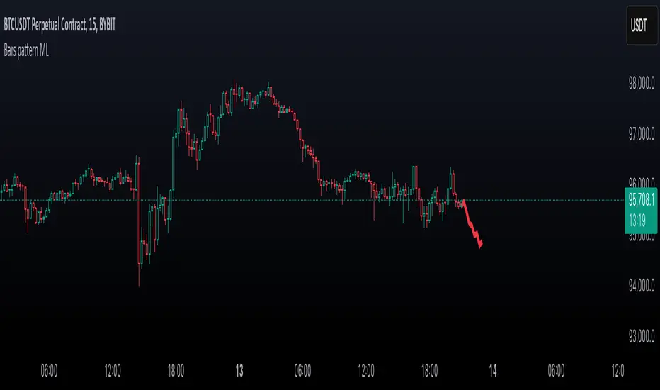
Bars pattern MLThis script implements a K-Nearest Neighbors (KNN)-based machine learning model to predict future price movements in financial markets. It analyzes past price action using Euclidean distance and selects the most similar historical patterns to estimate future price changes. Unlike traditional KNN implementations, this approach optimizes distance calculations by maintaining a dynamically updated list of the closest neighbors, ensuring efficient selection without the need for sorting. The model generates a forecasted price trajectory based on incremental predictions, which are visualized on the chart using polylines for better interpretability.
ค้นหาในสคริปต์สำหรับ "bar"
Volume HighlightBar colouring: this indicator is simple but effective, it repaints higher than normal candles a certain colour (by default gold/yellow) it helps to know what are valuable areas to trade around for longs and shorts.
Changing the volume multiplier manually helps you to screen volume relevant to the timeframe you are trading on.
For example, some charts 1min the best filter/setting would be 12-35 multiplier where others like btc 1-4 hourly, the filter/setting might be 8-12.
The key is having only the highest/most relevant 3-4 volume candles showing as they often represent supports and resistances.


Pivot Points And Breakout Price Action With LuckyNickVaBar Color Candle Aligned with pivot points swing high and swing lows For Those Who Are Familiar with Trading The Breakouts Of Highs & Lows Of Structure. Pivots are said to be key areas in the market where price shows heavy reaction to where reversals make occur. At these points there are swing Highs & swing lows that traders may be able to find opportunity in the market. This Script is a combination of pivot points and Barcolor signals for the breakout.

Koalafied Volume Extension Bar colours based on extensions from volume Z-Score. Large volume candles can often signal exhaustion or show market strength in reversals or breakouts. Candles not supported by rising volume are coloured black while those that are retain their colouring.

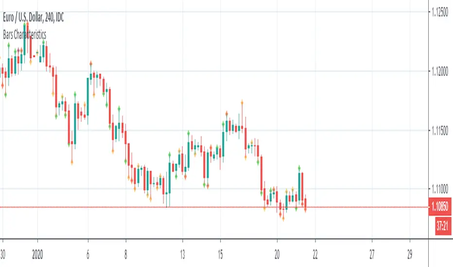
Bars CharacteristicsThis code is for defining or explaining market conditions via micro trend and the characterized bars.
lines 5,6: show the conditions for a normal trend, means market can go in the direction that it has in the past.
lines 11,12: show the conditions for kind of the trend having cumulative energy itself, mean market can go in the same direction.
lines 18,19: show the conditions for kind of the trend having overbought/sold concept, means it's better exit from the market or to look for the other clues.
lines 24,25: show some kind of noise not a stable trend, it's better not to enter the market.

WhenWasThePriceAction
Bars of largest range (volatility)
* see moments of strongest price action immediately
* colored & upDown by candle color
* amplifier: you see only the bull runs, and subsequent dumps
Very nice on the 5 years scale of BITSTAMP:BTCUSD - nothing comparable to 2013 has happened yet.
Internals:
squared_range = pow(high-low, 2)
That is essentially it already. The rest are details:
* gauge with (in case of Bitcoin exponentially rising) price
* show in red for negative candles
* take even higher polynomial (than 2) to show only the very largest values
* allow some user input (but there is not much more that can be chosen here.)
Sorry for such a simple formula - but sometimes the easiest things are powerful.
Please give feedback. www.tradingview.com and/or in the cryptocurrency chat. Thanks.


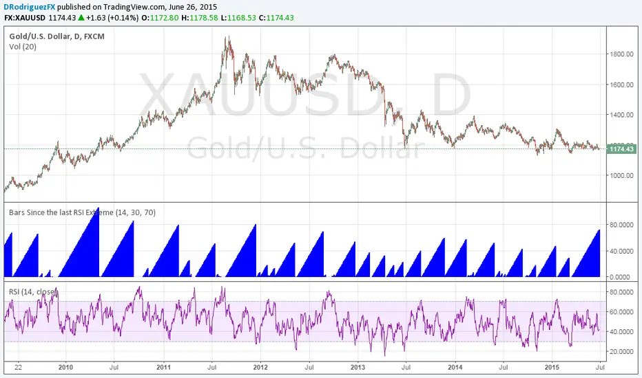
Bars Since the last RSI ExtremeThis is something Jamie Saettele pointed out. Gold has been in 'neutral' RSI territory for its longest stretch in four years. It's coiling up for its next major move.
Volume Candle Coloring v5 (BARCOLOR STABLE)Volume Candle Coloring v5 (Barcolor Stable) is a TradingView indicator that dynamically colors price candles based on relative volume intensity and candle direction.
The indicator compares the current volume to a moving average of volume and classifies it into five distinct levels: Low, Normal, High, Extreme, and Ultra. Each level is mapped to a clear, stable color scheme, ensuring excellent readability and no repainting or color flickering.
Bullish and bearish candles are colored separately, allowing traders to instantly identify:
Strong buying pressure
Strong selling pressure
Volume exhaustion
Low-interest / ranging conditions
The color priority is strictly ordered to guarantee stable bar coloring across all market conditions.
🔧 Key Features
Volume-based candle coloring using a moving average reference
Five volume intensity levels (Low → Ultra)
Separate color sets for bullish and bearish candles
Stable barcolor logic (no repainting, no shifting)
Fully customizable volume thresholds
Works on all markets and timeframes
🎯 Use Cases
Identify high-conviction breakouts
Spot volume climaxes and exhaustion
Confirm trend strength
Improve price action and volume analysis
⚙️ Inputs
Volume MA Period
Low / High / Extreme / Ultra volume multipliers

BarCoreLibrary "BarCore"
BarCore is a foundational library for technical analysis, providing essential functions for evaluating the structural properties of candlesticks and inter-bar relationships.
It prioritizes ratio-based metrics (0.0 to 1.0) over absolute prices, making it asset-agnostic and ideal for robust pattern recognition, momentum analysis, and volume-weighted pressure evaluation.
Key modules:
- Structure & Range: High-precision bar and body metrics with relative positioning.
- Wick Dynamics: Absolute and relative wick analysis for identifying price rejection.
- Inter-bar Logic: Containment, coverage, and quantitative price overlap (Ratio-based).
- Gap Intelligence: Real body and price gaps with customizable significance thresholds.
- Flow & Pressure: Volume-weighted buying/selling pressure and Money Flow metrics.
isBuyingBar()
Checks if the bar is a bullish (up) bar, where close is greater than open.
Returns: bool True if the bar closed higher than it opened.
isSellingBar()
Checks if the bar is a bearish (down) bar, where close is less than open.
Returns: bool True if the bar closed lower than it opened.
barMidpoint()
Calculates the absolute midpoint of the bar's total range (High + Low) / 2.
Returns: float The midpoint price of the bar.
barRange()
Calculates the absolute size of the bar's total range (High to Low).
Returns: float The absolute difference between high and low.
barRangeMidpoint()
Calculates half of the bar's total range size.
Returns: float Half the bar's range size.
realBodyHigh()
Returns the higher price between the open and close.
Returns: float The top of the real body.
realBodyLow()
Returns the lower price between the open and close.
Returns: float The bottom of the real body.
realBodyMidpoint()
Calculates the absolute midpoint of the bar's real body.
Returns: float The midpoint price of the real body.
realBodyRange()
Calculates the absolute size of the bar's real body.
Returns: float The absolute difference between open and close.
realBodyRangeMidpoint()
Calculates half of the bar's real body size.
Returns: float Half the real body size.
upperWickRange()
Calculates the absolute size of the upper wick.
Returns: float The range from high to the real body high.
lowerWickRange()
Calculates the absolute size of the lower wick.
Returns: float The range from the real body low to low.
openRatio()
Returns the location of the open price relative to the bar's total range (0.0 at low to 1.0 at high).
Returns: float The ratio of the distance from low to open, divided by the total range.
closeRatio()
Returns the location of the close price relative to the bar's total range (0.0 at low to 1.0 at high).
Returns: float The ratio of the distance from low to close, divided by the total range.
realBodyRatio()
Calculates the ratio of the real body size to the total bar range.
Returns: float The real body size divided by the bar range. Returns 0 if barRange is 0.
upperWickRatio()
Calculates the ratio of the upper wick size to the total bar range.
Returns: float The upper wick size divided by the bar range. Returns 0 if barRange is 0.
lowerWickRatio()
Calculates the ratio of the lower wick size to the total bar range.
Returns: float The lower wick size divided by the bar range. Returns 0 if barRange is 0.
upperWickToBodyRatio()
Calculates the ratio of the upper wick size to the real body size.
Returns: float The upper wick size divided by the real body size. Returns 0 if realBodyRange is 0.
lowerWickToBodyRatio()
Calculates the ratio of the lower wick size to the real body size.
Returns: float The lower wick size divided by the real body size. Returns 0 if realBodyRange is 0.
totalWickRatio()
Calculates the ratio of the total wick range (Upper Wick + Lower Wick) to the total bar range.
Returns: float The total wick range expressed as a ratio of the bar's total range. Returns 0 if barRange is 0.
isBodyExpansion()
Checks if the current bar's real body range is larger than the previous bar's real body range (body expansion).
Returns: bool True if realBodyRange() > realBodyRange() .
isBodyContraction()
Checks if the current bar's real body range is smaller than the previous bar's real body range (body contraction).
Returns: bool True if realBodyRange() < realBodyRange() .
isWithinPrevBar(inclusive)
Checks if the current bar's range is entirely within the previous bar's range.
Parameters:
inclusive (bool) : If true, allows equality (<=, >=). Default is false.
Returns: bool True if High < High AND Low > Low .
isCoveringPrevBar(inclusive)
Checks if the current bar's range fully covers the entire previous bar's range.
Parameters:
inclusive (bool) : If true, allows equality (<=, >=). Default is false.
Returns: bool True if High > High AND Low < Low .
isWithinPrevBody(inclusive)
Checks if the current bar's real body is entirely inside the previous bar's real body.
Parameters:
inclusive (bool) : If true, allows equality (<=, >=). Default is false.
Returns: bool True if the current body is contained inside the previous body.
isCoveringPrevBody(inclusive)
Checks if the current bar's real body fully covers the previous bar's real body.
Parameters:
inclusive (bool) : If true, allows equality (<=, >=). Default is false.
Returns: bool True if the current body fully covers the previous body.
isOpenWithinPrevBody(inclusive)
Checks if the current bar's open price falls within the real body range of the previous bar.
Parameters:
inclusive (bool) : If true, includes the boundary prices. Default is false.
Returns: bool True if the open price is between the previous bar's real body high and real body low.
isCloseWithinPrevBody(inclusive)
Checks if the current bar's close price falls within the real body range of the previous bar.
Parameters:
inclusive (bool) : If true, includes the boundary prices. Default is false.
Returns: bool True if the close price is between the previous bar's real body high and real body low.
isPrevOpenWithinBody(inclusive)
Checks if the previous bar's open price falls within the current bar's real body range.
Parameters:
inclusive (bool) : If true, includes the boundary prices. Default is false.
Returns: bool True if open is between the current bar's real body high and real body low.
isPrevCloseWithinBody(inclusive)
Checks if the previous bar's closing price falls within the current bar's real body range.
Parameters:
inclusive (bool) : If true, includes the boundary prices. Default is false.
Returns: bool True if close is between the current bar's real body high and real body low.
isOverlappingPrevBar()
Checks if there is any price overlap between the current bar's range and the previous bar's range.
Returns: bool True if the current bar's range has any intersection with the previous bar's range.
bodyOverlapRatio()
Calculates the percentage of the current real body that overlaps with the previous real body.
Returns: float The overlap ratio (0.0 to 1.0). 1.0 means the current body is entirely within the previous body's price range.
isCompletePriceGapUp()
Checks for a complete price gap up where the current bar's low is strictly above the previous bar's high, meaning there is zero price overlap between the two bars.
Returns: bool True if the current low is greater than the previous high.
isCompletePriceGapDown()
Checks for a complete price gap down where the current bar's high is strictly below the previous bar's low, meaning there is zero price overlap between the two bars.
Returns: bool True if the current high is less than the previous low.
isRealBodyGapUp()
Checks for a gap between the current and previous real bodies.
Returns: bool True if the current body is completely above the previous body.
isRealBodyGapDown()
Checks for a gap between the current and previous real bodies.
Returns: bool True if the current body is completely below the previous body.
gapRatio()
Calculates the percentage difference between the current open and the previous close, expressed as a decimal ratio.
Returns: float The gap ratio (positive for gap up, negative for gap down). Returns 0 if the previous close is 0.
gapPercentage()
Calculates the percentage difference between the current open and the previous close.
Returns: float The gap percentage (positive for gap up, negative for gap down). Returns 0 if previous close is 0.
isGapUp()
Checks for a basic gap up, where the current bar's open is strictly higher than the previous bar's close. This is the minimum condition for a gap up.
Returns: bool True if the current open is greater than the previous close (i.e., gapRatio is positive).
isGapDown()
Checks for a basic gap down, where the current bar's open is strictly lower than the previous bar's close. This is the minimum condition for a gap down.
Returns: bool True if the current open is less than the previous close (i.e., gapRatio is negative).
isSignificantGapUp(minRatio)
Checks if the current bar opened significantly higher than the previous close, as defined by a minimum percentage ratio.
Parameters:
minRatio (float) : The minimum required gap percentage ratio. Default is 0.03 (3%).
Returns: bool True if the gap ratio (open vs. previous close) is greater than or equal to the minimum ratio.
isSignificantGapDown(minRatio)
Checks if the current bar opened significantly lower than the previous close, as defined by a minimum percentage ratio.
Parameters:
minRatio (float) : The minimum required gap percentage ratio. Default is 0.03 (3%).
Returns: bool True if the absolute value of the gap ratio (open vs. previous close) is greater than or equal to the minimum ratio.
trueRangeComponentHigh()
Calculates the absolute distance from the current bar's High to the previous bar's Close, representing one of the components of the True Range.
Returns: float The absolute difference: |High - Close |.
trueRangeComponentLow()
Calculates the absolute distance from the current bar's Low to the previous bar's Close, representing one of the components of the True Range.
Returns: float The absolute difference: |Low - Close |.
isUpperWickDominant(minRatio)
Checks if the upper wick is significantly long relative to the total range.
Parameters:
minRatio (float) : Minimum ratio of the wick to the total bar range. Default is 0.7 (70%).
Returns: bool True if the upper wick dominates the bar's range.
isUpperWickNegligible(maxRatio)
Checks if the upper wick is very small relative to the total range.
Parameters:
maxRatio (float) : Maximum ratio of the wick to the total bar range. Default is 0.05 (5%).
Returns: bool True if the upper wick is negligible.
isLowerWickDominant(minRatio)
Checks if the lower wick is significantly long relative to the total range.
Parameters:
minRatio (float) : Minimum ratio of the wick to the total bar range. Default is 0.7 (70%).
Returns: bool True if the lower wick dominates the bar's range.
isLowerWickNegligible(maxRatio)
Checks if the lower wick is very small relative to the total range.
Parameters:
maxRatio (float) : Maximum ratio of the wick to the total bar range. Default is 0.05 (5%).
Returns: bool True if the lower wick is negligible.
isSymmetric(maxTolerance)
Checks if the upper and lower wicks are roughly equal in length.
Parameters:
maxTolerance (float) : Maximum allowable percentage difference between the two wicks. Default is 0.15 (15%).
Returns: bool True if wicks are symmetric within the tolerance level.
isMarubozuBody(minRatio)
Candle with a very large body relative to the total range (minimal wicks).
Parameters:
minRatio (float) : Minimum body size ratio. Default is 0.9 (90%).
Returns: bool True if the bar has minimal wicks (Marubozu body).
isLargeBody(minRatio)
Candle with a large body relative to the total range.
Parameters:
minRatio (float) : Minimum body size ratio. Default is 0.6 (60%).
Returns: bool True if the bar has a large body.
isSmallBody(maxRatio)
Candle with a small body relative to the total range.
Parameters:
maxRatio (float) : Maximum body size ratio. Default is 0.4 (40%).
Returns: bool True if the bar has small body.
isDojiBody(maxRatio)
Candle with a very small body relative to the total range (indecision).
Parameters:
maxRatio (float) : Maximum body size ratio. Default is 0.1 (10%).
Returns: bool True if the bar has a very small body.
isLowerWickExtended(minRatio)
Checks if the lower wick is significantly extended relative to the real body size.
Parameters:
minRatio (float) : Minimum required ratio of the lower wick length to the real body size. Default is 2.0 (Lower wick must be at least twice the body's size).
Returns: bool True if the lower wick's length is at least `minRatio` times the size of the real body.
isUpperWickExtended(minRatio)
Checks if the upper wick is significantly extended relative to the real body size.
Parameters:
minRatio (float) : Minimum required ratio of the upper wick length to the real body size. Default is 2.0 (Upper wick must be at least twice the body's size).
Returns: bool True if the upper wick's length is at least `minRatio` times the size of the real body.
isStrongBuyingBar(minCloseRatio, maxOpenRatio)
Checks for a bar with strong bullish momentum (open near low, close near high), indicating high conviction.
Parameters:
minCloseRatio (float) : Minimum required ratio for the close location (relative to range, e.g., 0.7 means close must be in the top 30%). Default is 0.7 (70%).
maxOpenRatio (float) : Maximum allowed ratio for the open location (relative to range, e.g., 0.3 means open must be in the bottom 30%). Default is 0.3 (30%).
Returns: bool True if the bar is bullish, opened in the low extreme, and closed in the high extreme.
isStrongSellingBar(maxCloseRatio, minOpenRatio)
Checks for a bar with strong bearish momentum (open near high, close near low), indicating high conviction.
Parameters:
maxCloseRatio (float) : Maximum allowed ratio for the close location (relative to range, e.g., 0.3 means close must be in the bottom 30%). Default is 0.3 (30%).
minOpenRatio (float) : Minimum required ratio for the open location (relative to range, e.g., 0.7 means open must be in the top 30%). Default is 0.7 (70%).
Returns: bool True if the bar is bearish, opened in the high extreme, and closed in the low extreme.
isWeakBuyingBar(maxCloseRatio, maxBodyRatio)
Identifies a bar that is technically bullish but shows significant weakness, characterized by a failure to close near the high and a small body size.
Parameters:
maxCloseRatio (float) : Maximum allowed ratio for the close location relative to the range (e.g., 0.6 means the close must be in the bottom 60% of the bar's range). Default is 0.6 (60%).
maxBodyRatio (float) : Maximum allowed ratio for the real body size relative to the bar's range (e.g., 0.4 means the body is small). Default is 0.4 (40%).
Returns: bool True if the bar is bullish, but its close is weak and its body is small.
isWeakSellingBar(minCloseRatio, maxBodyRatio)
Identifies a bar that is technically bearish but shows significant weakness, characterized by a failure to close near the low and a small body size.
Parameters:
minCloseRatio (float) : Minimum required ratio for the close location relative to the range (e.g., 0.4 means the close must be in the top 60% of the bar's range). Default is 0.4 (40%).
maxBodyRatio (float) : Maximum allowed ratio for the real body size relative to the bar's range (e.g., 0.4 means the body is small). Default is 0.4 (40%).
Returns: bool True if the bar is bearish, but its close is weak and its body is small.
balanceOfPower()
Measures the net pressure of buyers vs. sellers within the bar, normalized to the bar's range.
Returns: float A value between -1.0 (strong selling) and +1.0 (strong buying), representing the strength and direction of the close relative to the open.
buyingPressure()
Measures the net buying volume pressure based on the close location and volume.
Returns: float A numerical value representing the volume weighted buying pressure.
sellingPressure()
Measures the net selling volume pressure based on the close location and volume.
Returns: float A numerical value representing the volume weighted selling pressure.
moneyFlowMultiplier()
Calculates the Money Flow Multiplier (MFM), which is the price component of Money Flow and CMF.
Returns: float A normalized value from -1.0 (strong selling) to +1.0 (strong buying), representing the net directional pressure.
moneyFlowVolume()
Calculates the Money Flow Volume (MFV), which is the Money Flow Multiplier weighted by the bar's volume.
Returns: float A numerical value representing the volume-weighted money flow. Positive = buying dominance; negative = selling dominance.
isAccumulationBar()
Checks for basic accumulation on the current bar, requiring both positive Money Flow Volume and a buying bar (closing higher than opening).
Returns: bool True if the bar exhibits buying dominance through its internal range location and is a buying bar.
isDistributionBar()
Checks for basic distribution on the current bar, requiring both negative Money Flow Volume and a selling bar (closing lower than opening).
Returns: bool True if the bar exhibits selling dominance through its internal range location and is a selling bar.

Adaptive Genesis Engine [AGE]ADAPTIVE GENESIS ENGINE (AGE)
Pure Signal Evolution Through Genetic Algorithms
Where Darwin Meets Technical Analysis
🧬 WHAT YOU'RE GETTING - THE PURE INDICATOR
This is a technical analysis indicator - it generates signals, visualizes probability, and shows you the evolutionary process in real-time. This is NOT a strategy with automatic execution - it's a sophisticated signal generation system that you control .
What This Indicator Does:
Generates Long/Short entry signals with probability scores (35-88% range)
Evolves a population of up to 12 competing strategies using genetic algorithms
Validates strategies through walk-forward optimization (train/test cycles)
Visualizes signal quality through premium gradient clouds and confidence halos
Displays comprehensive metrics via enhanced dashboard
Provides alerts for entries and exits
Works on any timeframe, any instrument, any broker
What This Indicator Does NOT Do:
Execute trades automatically
Manage positions or calculate position sizes
Place orders on your behalf
Make trading decisions for you
This is pure signal intelligence. AGE tells you when and how confident it is. You decide whether and how much to trade.
🔬 THE SCIENCE: GENETIC ALGORITHMS MEET TECHNICAL ANALYSIS
What Makes This Different - The Evolutionary Foundation
Most indicators are static - they use the same parameters forever, regardless of market conditions. AGE is alive . It maintains a population of competing strategies that evolve, adapt, and improve through natural selection principles:
Birth: New strategies spawn through crossover breeding (combining DNA from fit parents) plus random mutation for exploration
Life: Each strategy trades virtually via shadow portfolios, accumulating wins/losses, tracking drawdown, and building performance history
Selection: Strategies are ranked by comprehensive fitness scoring (win rate, expectancy, drawdown control, signal efficiency)
Death: Weak strategies are culled periodically, with elite performers (top 2 by default) protected from removal
Evolution: The gene pool continuously improves as successful traits propagate and unsuccessful ones die out
This is not curve-fitting. Each new strategy must prove itself on out-of-sample data through walk-forward validation before being trusted for live signals.
🧪 THE DNA: WHAT EVOLVES
Every strategy carries a 10-gene chromosome controlling how it interprets market data:
Signal Sensitivity Genes
Entropy Sensitivity (0.5-2.0): Weight given to market order/disorder calculations. Low values = conservative, require strong directional clarity. High values = aggressive, act on weaker order signals.
Momentum Sensitivity (0.5-2.0): Weight given to RSI/ROC/MACD composite. Controls responsiveness to momentum shifts vs. mean-reversion setups.
Structure Sensitivity (0.5-2.0): Weight given to support/resistance positioning. Determines how much price location within swing range matters.
Probability Adjustment Genes
Probability Boost (-0.10 to +0.10): Inherent bias toward aggressive (+) or conservative (-) entries. Acts as personality trait - some strategies naturally optimistic, others pessimistic.
Trend Strength Requirement (0.3-0.8): Minimum trend conviction needed before signaling. Higher values = only trades strong trends, lower values = acts in weak/sideways markets.
Volume Filter (0.5-1.5): Strictness of volume confirmation. Higher values = requires strong volume, lower values = volume less important.
Risk Management Genes
ATR Multiplier (1.5-4.0): Base volatility scaling for all price levels. Controls whether strategy uses tight or wide stops/targets relative to ATR.
Stop Multiplier (1.0-2.5): Stop loss tightness. Lower values = aggressive profit protection, higher values = more breathing room.
Target Multiplier (1.5-4.0): Profit target ambition. Lower values = quick scalping exits, higher values = swing trading holds.
Adaptation Gene
Regime Adaptation (0.0-1.0): How much strategy adjusts behavior based on detected market regime (trending/volatile/choppy). Higher values = more reactive to regime changes.
The Magic: AGE doesn't just try random combinations. Through tournament selection and fitness-weighted crossover, successful gene combinations spread through the population while unsuccessful ones fade away. Over 50-100 bars, you'll see the population converge toward genes that work for YOUR instrument and timeframe.
📊 THE SIGNAL ENGINE: THREE-LAYER SYNTHESIS
Before any strategy generates a signal, AGE calculates probability through multi-indicator confluence:
Layer 1 - Market Entropy (Information Theory)
Measures whether price movements exhibit directional order or random walk characteristics:
The Math:
Shannon Entropy = -Σ(p × log(p))
Market Order = 1 - (Entropy / 0.693)
What It Means:
High entropy = choppy, random market → low confidence signals
Low entropy = directional market → high confidence signals
Direction determined by up-move vs down-move dominance over lookback period (default: 20 bars)
Signal Output: -1.0 to +1.0 (bearish order to bullish order)
Layer 2 - Momentum Synthesis
Combines three momentum indicators into single composite score:
Components:
RSI (40% weight): Normalized to -1/+1 scale using (RSI-50)/50
Rate of Change (30% weight): Percentage change over lookback (default: 14 bars), clamped to ±1
MACD Histogram (30% weight): Fast(12) - Slow(26), normalized by ATR
Why This Matters: RSI catches mean-reversion opportunities, ROC catches raw momentum, MACD catches momentum divergence. Weighting favors RSI for reliability while keeping other perspectives.
Signal Output: -1.0 to +1.0 (strong bearish to strong bullish)
Layer 3 - Structure Analysis
Evaluates price position within swing range (default: 50-bar lookback):
Position Classification:
Bottom 20% of range = Support Zone → bullish bounce potential
Top 20% of range = Resistance Zone → bearish rejection potential
Middle 60% = Neutral Zone → breakout/breakdown monitoring
Signal Logic:
At support + bullish candle = +0.7 (strong buy setup)
At resistance + bearish candle = -0.7 (strong sell setup)
Breaking above range highs = +0.5 (breakout confirmation)
Breaking below range lows = -0.5 (breakdown confirmation)
Consolidation within range = ±0.3 (weak directional bias)
Signal Output: -1.0 to +1.0 (bearish structure to bullish structure)
Confluence Voting System
Each layer casts a vote (Long/Short/Neutral). The system requires minimum 2-of-3 agreement (configurable 1-3) before generating a signal:
Examples:
Entropy: Bullish, Momentum: Bullish, Structure: Neutral → Signal generated (2 long votes)
Entropy: Bearish, Momentum: Neutral, Structure: Neutral → No signal (only 1 short vote)
All three bullish → Signal generated with +5% probability bonus
This is the key to quality. Single indicators give too many false signals. Triple confirmation dramatically improves accuracy.
📈 PROBABILITY CALCULATION: HOW CONFIDENCE IS MEASURED
Base Probability:
Raw_Prob = 50% + (Average_Signal_Strength × 25%)
Then AGE applies strategic adjustments:
Trend Alignment:
Signal with trend: +4%
Signal against strong trend: -8%
Weak/no trend: no adjustment
Regime Adaptation:
Trending market (efficiency >50%, moderate vol): +3%
Volatile market (vol ratio >1.5x): -5%
Choppy market (low efficiency): -2%
Volume Confirmation:
Volume > 70% of 20-bar SMA: no change
Volume below threshold: -3%
Volatility State (DVS Ratio):
High vol (>1.8x baseline): -4% (reduce confidence in chaos)
Low vol (<0.7x baseline): -2% (markets can whipsaw in compression)
Moderate elevated vol (1.0-1.3x): +2% (trending conditions emerging)
Confluence Bonus:
All 3 indicators agree: +5%
2 of 3 agree: +2%
Strategy Gene Adjustment:
Probability Boost gene: -10% to +10%
Regime Adaptation gene: scales regime adjustments by 0-100%
Final Probability: Clamped between 35% (minimum) and 88% (maximum)
Why These Ranges?
Below 35% = too uncertain, better not to signal
Above 88% = unrealistic, creates overconfidence
Sweet spot: 65-80% for quality entries
🔄 THE SHADOW PORTFOLIO SYSTEM: HOW STRATEGIES COMPETE
Each active strategy maintains a virtual trading account that executes in parallel with real-time data:
Shadow Trading Mechanics
Entry Logic:
Calculate signal direction, probability, and confluence using strategy's unique DNA
Check if signal meets quality gate:
Probability ≥ configured minimum threshold (default: 65%)
Confluence ≥ configured minimum (default: 2 of 3)
Direction is not zero (must be long or short, not neutral)
Verify signal persistence:
Base requirement: 2 bars (configurable 1-5)
Adapts based on probability: high-prob signals (75%+) enter 1 bar faster, low-prob signals need 1 bar more
Adjusts for regime: trending markets reduce persistence by 1, volatile markets add 1
Apply additional filters:
Trend strength must exceed strategy's requirement gene
Regime filter: if volatile market detected, probability must be 72%+ to override
Volume confirmation required (volume > 70% of average)
If all conditions met for required persistence bars, enter shadow position at current close price
Position Management:
Entry Price: Recorded at close of entry bar
Stop Loss: ATR-based distance = ATR × ATR_Mult (gene) × Stop_Mult (gene) × DVS_Ratio
Take Profit: ATR-based distance = ATR × ATR_Mult (gene) × Target_Mult (gene) × DVS_Ratio
Position: +1 (long) or -1 (short), only one at a time per strategy
Exit Logic:
Check if price hit stop (on low) or target (on high) on current bar
Record trade outcome in R-multiples (profit/loss normalized by ATR)
Update performance metrics:
Total trades counter incremented
Wins counter (if profit > 0)
Cumulative P&L updated
Peak equity tracked (for drawdown calculation)
Maximum drawdown from peak recorded
Enter cooldown period (default: 8 bars, configurable 3-20) before next entry allowed
Reset signal age counter to zero
Walk-Forward Tracking:
During position lifecycle, trades are categorized:
Training Phase (first 250 bars): Trade counted toward training metrics
Testing Phase (next 75 bars): Trade counted toward testing metrics (out-of-sample)
Live Phase (after WFO period): Trade counted toward overall metrics
Why Shadow Portfolios?
No lookahead bias (uses only data available at the bar)
Realistic execution simulation (entry on close, stop/target checks on high/low)
Independent performance tracking for true fitness comparison
Allows safe experimentation without risking capital
Each strategy learns from its own experience
🏆 FITNESS SCORING: HOW STRATEGIES ARE RANKED
Fitness is not just win rate. AGE uses a comprehensive multi-factor scoring system:
Core Metrics (Minimum 3 trades required)
Win Rate (30% of fitness):
WinRate = Wins / TotalTrades
Normalized directly (0.0-1.0 scale)
Total P&L (30% of fitness):
Normalized_PnL = (PnL + 300) / 600
Clamped 0.0-1.0. Assumes P&L range of -300R to +300R for normalization scale.
Expectancy (25% of fitness):
Expectancy = Total_PnL / Total_Trades
Normalized_Expectancy = (Expectancy + 30) / 60
Clamped 0.0-1.0. Rewards consistency of profit per trade.
Drawdown Control (15% of fitness):
Normalized_DD = 1 - (Max_Drawdown / 15)
Clamped 0.0-1.0. Penalizes strategies that suffer large equity retracements from peak.
Sample Size Adjustment
Quality Factor:
<50 trades: 1.0 (full weight, small sample)
50-100 trades: 0.95 (slight penalty for medium sample)
100 trades: 0.85 (larger penalty for large sample)
Why penalize more trades? Prevents strategies from gaming the system by taking hundreds of tiny trades to inflate statistics. Favors quality over quantity.
Bonus Adjustments
Walk-Forward Validation Bonus:
if (WFO_Validated):
Fitness += (WFO_Efficiency - 0.5) × 0.1
Strategies proven on out-of-sample data receive up to +10% fitness boost based on test/train efficiency ratio.
Signal Efficiency Bonus (if diagnostics enabled):
if (Signals_Evaluated > 10):
Pass_Rate = Signals_Passed / Signals_Evaluated
Fitness += (Pass_Rate - 0.1) × 0.05
Rewards strategies that generate high-quality signals passing the quality gate, not just profitable trades.
Final Fitness: Clamped at 0.0 minimum (prevents negative fitness values)
Result: Elite strategies typically achieve 0.50-0.75 fitness. Anything above 0.60 is excellent. Below 0.30 is prime candidate for culling.
🔬 WALK-FORWARD OPTIMIZATION: ANTI-OVERFITTING PROTECTION
This is what separates AGE from curve-fitted garbage indicators.
The Three-Phase Process
Every new strategy undergoes a rigorous validation lifecycle:
Phase 1 - Training Window (First 250 bars, configurable 100-500):
Strategy trades normally via shadow portfolio
All trades count toward training performance metrics
System learns which gene combinations produce profitable patterns
Tracks independently: Training_Trades, Training_Wins, Training_PnL
Phase 2 - Testing Window (Next 75 bars, configurable 30-200):
Strategy continues trading without any parameter changes
Trades now count toward testing performance metrics (separate tracking)
This is out-of-sample data - strategy has never seen these bars during "optimization"
Tracks independently: Testing_Trades, Testing_Wins, Testing_PnL
Phase 3 - Validation Check:
Minimum_Trades = 5 (configurable 3-15)
IF (Train_Trades >= Minimum AND Test_Trades >= Minimum):
WR_Efficiency = Test_WinRate / Train_WinRate
Expectancy_Efficiency = Test_Expectancy / Train_Expectancy
WFO_Efficiency = (WR_Efficiency + Expectancy_Efficiency) / 2
IF (WFO_Efficiency >= 0.55): // configurable 0.3-0.9
Strategy.Validated = TRUE
Strategy receives fitness bonus
ELSE:
Strategy receives 30% fitness penalty
ELSE:
Validation deferred (insufficient trades in one or both periods)
What Validation Means
Validated Strategy (Green "✓ VAL" in dashboard):
Performed at least 55% as well on unseen data compared to training data
Gets fitness bonus: +(efficiency - 0.5) × 0.1
Receives priority during tournament selection for breeding
More likely to be chosen as active trading strategy
Unvalidated Strategy (Orange "○ TRAIN" in dashboard):
Failed to maintain performance on test data (likely curve-fitted to training period)
Receives 30% fitness penalty (0.7x multiplier)
Makes strategy prime candidate for culling
Can still trade but with lower selection probability
Insufficient Data (continues collecting):
Hasn't completed both training and testing periods yet
OR hasn't achieved minimum trade count in both periods
Validation check deferred until requirements met
Why 55% Efficiency Threshold?
If a strategy earned 10R during training but only 5.5R during testing, it still proved an edge exists beyond random luck. Requiring 100% efficiency would be unrealistic - market conditions change between periods. But requiring >50% ensures the strategy didn't completely degrade on fresh data.
The Protection: Strategies that work great on historical data but fail on new data are automatically identified and penalized. This prevents the population from being polluted by overfitted strategies that would fail in live trading.
🌊 DYNAMIC VOLATILITY SCALING (DVS): ADAPTIVE STOP/TARGET PLACEMENT
AGE doesn't use fixed stop distances. It adapts to current volatility conditions in real-time.
Four Volatility Measurement Methods
1. ATR Ratio (Simple Method):
Current_Vol = ATR(14) / Close
Baseline_Vol = SMA(Current_Vol, 100)
Ratio = Current_Vol / Baseline_Vol
Basic comparison of current ATR to 100-bar moving average baseline.
2. Parkinson (High-Low Range Based):
For each bar: HL = log(High / Low)
Parkinson_Vol = sqrt(Σ(HL²) / (4 × Period × log(2)))
More stable than close-to-close volatility. Captures intraday range expansion without overnight gap noise.
3. Garman-Klass (OHLC Based):
HL_Term = 0.5 × ²
CO_Term = (2×log(2) - 1) × ²
GK_Vol = sqrt(Σ(HL_Term - CO_Term) / Period)
Most sophisticated estimator. Incorporates all four price points (open, high, low, close) plus gap information.
4. Ensemble Method (Default - Median of All Three):
Ratio_1 = ATR_Current / ATR_Baseline
Ratio_2 = Parkinson_Current / Parkinson_Baseline
Ratio_3 = GK_Current / GK_Baseline
DVS_Ratio = Median(Ratio_1, Ratio_2, Ratio_3)
Why Ensemble?
Takes median to avoid outliers and false spikes
If ATR jumps but range-based methods stay calm, median prevents overreaction
If one method fails, other two compensate
Most robust approach across different market conditions
Sensitivity Scaling
Scaled_Ratio = (Raw_Ratio) ^ Sensitivity
Sensitivity 0.3: Cube root - heavily dampens volatility impact
Sensitivity 0.5: Square root - moderate dampening
Sensitivity 0.7 (Default): Balanced response to volatility changes
Sensitivity 1.0: Linear - full 1:1 volatility impact
Sensitivity 1.5: Exponential - amplified response to volatility spikes
Safety Clamps: Final DVS Ratio always clamped between 0.5x and 2.5x baseline to prevent extreme position sizing or stop placement errors.
How DVS Affects Shadow Trading
Every strategy's stop and target distances are multiplied by the current DVS ratio:
Stop Loss Distance:
Stop_Distance = ATR × ATR_Mult (gene) × Stop_Mult (gene) × DVS_Ratio
Take Profit Distance:
Target_Distance = ATR × ATR_Mult (gene) × Target_Mult (gene) × DVS_Ratio
Example Scenario:
ATR = 10 points
Strategy's ATR_Mult gene = 2.5
Strategy's Stop_Mult gene = 1.5
Strategy's Target_Mult gene = 2.5
DVS_Ratio = 1.4 (40% above baseline volatility - market heating up)
Stop = 10 × 2.5 × 1.5 × 1.4 = 52.5 points (vs. 37.5 in normal vol)
Target = 10 × 2.5 × 2.5 × 1.4 = 87.5 points (vs. 62.5 in normal vol)
Result:
During volatility spikes: Stops automatically widen to avoid noise-based exits, targets extend for bigger moves
During calm periods: Stops tighten for better risk/reward, targets compress for realistic profit-taking
Strategies adapt risk management to match current market behavior
🧬 THE EVOLUTIONARY CYCLE: SPAWN, COMPETE, CULL
Initialization (Bar 1)
AGE begins with 4 seed strategies (if evolution enabled):
Seed Strategy #0 (Balanced):
All sensitivities at 1.0 (neutral)
Zero probability boost
Moderate trend requirement (0.4)
Standard ATR/stop/target multiples (2.5/1.5/2.5)
Mid-level regime adaptation (0.5)
Seed Strategy #1 (Momentum-Focused):
Lower entropy sensitivity (0.7), higher momentum (1.5)
Slight probability boost (+0.03)
Higher trend requirement (0.5)
Tighter stops (1.3), wider targets (3.0)
Seed Strategy #2 (Entropy-Driven):
Higher entropy sensitivity (1.5), lower momentum (0.8)
Slight probability penalty (-0.02)
More trend tolerant (0.6)
Wider stops (1.8), standard targets (2.5)
Seed Strategy #3 (Structure-Based):
Balanced entropy/momentum (0.8/0.9), high structure (1.4)
Slight probability boost (+0.02)
Lower trend requirement (0.35)
Moderate risk parameters (1.6/2.8)
All seeds start with WFO validation bypassed if WFO is disabled, or must validate if enabled.
Spawning New Strategies
Timing (Adaptive):
Historical phase: Every 30 bars (configurable 10-100)
Live phase: Every 200 bars (configurable 100-500)
Automatically switches to live timing when barstate.isrealtime triggers
Conditions:
Current population < max population limit (default: 8, configurable 4-12)
At least 2 active strategies exist (need parents)
Available slot in population array
Selection Process:
Run tournament selection 3 times with different seeds
Each tournament: randomly sample active strategies, pick highest fitness
Best from 3 tournaments becomes Parent 1
Repeat independently for Parent 2
Ensures fit parents but maintains diversity
Crossover Breeding:
For each of 10 genes:
Parent1_Fitness = fitness
Parent2_Fitness = fitness
Weight1 = Parent1_Fitness / (Parent1_Fitness + Parent2_Fitness)
Gene1 = parent1's value
Gene2 = parent2's value
Child_Gene = Weight1 × Gene1 + (1 - Weight1) × Gene2
Fitness-weighted crossover ensures fitter parent contributes more genetic material.
Mutation:
For each gene in child:
IF (random < mutation_rate):
Gene_Range = GENE_MAX - GENE_MIN
Noise = (random - 0.5) × 2 × mutation_strength × Gene_Range
Mutated_Gene = Clamp(Child_Gene + Noise, GENE_MIN, GENE_MAX)
Historical mutation rate: 20% (aggressive exploration)
Live mutation rate: 8% (conservative stability)
Mutation strength: 12% of gene range (configurable 5-25%)
Initialization of New Strategy:
Unique ID assigned (total_spawned counter)
Parent ID recorded
Generation = max(parent generations) + 1
Birth bar recorded (for age tracking)
All performance metrics zeroed
Shadow portfolio reset
WFO validation flag set to false (must prove itself)
Result: New strategy with hybrid DNA enters population, begins trading in next bar.
Competition (Every Bar)
All active strategies:
Calculate their signal based on unique DNA
Check quality gate with their thresholds
Manage shadow positions (entries/exits)
Update performance metrics
Recalculate fitness score
Track WFO validation progress
Strategies compete indirectly through fitness ranking - no direct interaction.
Culling Weak Strategies
Timing (Adaptive):
Historical phase: Every 60 bars (configurable 20-200, should be 2x spawn interval)
Live phase: Every 400 bars (configurable 200-1000, should be 2x spawn interval)
Minimum Adaptation Score (MAS):
Initial MAS = 0.10
MAS decays: MAS × 0.995 every cull cycle
Minimum MAS = 0.03 (floor)
MAS represents the "survival threshold" - strategies below this fitness level are vulnerable.
Culling Conditions (ALL must be true):
Population > minimum population (default: 3, configurable 2-4)
At least one strategy has fitness < MAS
Strategy's age > culling interval (prevents premature culling of new strategies)
Strategy is not in top N elite (default: 2, configurable 1-3)
Culling Process:
Find worst strategy:
For each active strategy:
IF (age > cull_interval):
Fitness = base_fitness
IF (not WFO_validated AND WFO_enabled):
Fitness × 0.7 // 30% penalty for unvalidated
IF (Fitness < MAS AND Fitness < worst_fitness_found):
worst_strategy = this_strategy
worst_fitness = Fitness
IF (worst_strategy found):
Count elite strategies with fitness > worst_fitness
IF (elite_count >= elite_preservation_count):
Deactivate worst_strategy (set active flag = false)
Increment total_culled counter
Elite Protection:
Even if a strategy's fitness falls below MAS, it survives if fewer than N strategies are better. This prevents culling when population is generally weak.
Result: Weak strategies removed from population, freeing slots for new spawns. Gene pool improves over time.
Selection for Display (Every Bar)
AGE chooses one strategy to display signals:
Best fitness = -1
Selected = none
For each active strategy:
Fitness = base_fitness
IF (WFO_validated):
Fitness × 1.3 // 30% bonus for validated strategies
IF (Fitness > best_fitness):
best_fitness = Fitness
selected_strategy = this_strategy
Display selected strategy's signals on chart
Result: Only the highest-fitness (optionally validated-boosted) strategy's signals appear as chart markers. Other strategies trade invisibly in shadow portfolios.
🎨 PREMIUM VISUALIZATION SYSTEM
AGE includes sophisticated visual feedback that standard indicators lack:
1. Gradient Probability Cloud (Optional, Default: ON)
Multi-layer gradient showing signal buildup 2-3 bars before entry:
Activation Conditions:
Signal persistence > 0 (same directional signal held for multiple bars)
Signal probability ≥ minimum threshold (65% by default)
Signal hasn't yet executed (still in "forming" state)
Visual Construction:
7 gradient layers by default (configurable 3-15)
Each layer is a line-fill pair (top line, bottom line, filled between)
Layer spacing: 0.3 to 1.0 × ATR above/below price
Outer layers = faint, inner layers = bright
Color transitions from base to intense based on layer position
Transparency scales with probability (high prob = more opaque)
Color Selection:
Long signals: Gradient from theme.gradient_bull_mid to theme.gradient_bull_strong
Short signals: Gradient from theme.gradient_bear_mid to theme.gradient_bear_strong
Base transparency: 92%, reduces by up to 8% for high-probability setups
Dynamic Behavior:
Cloud grows/shrinks as signal persistence increases/decreases
Redraws every bar while signal is forming
Disappears when signal executes or invalidates
Performance Note: Computationally expensive due to linefill objects. Disable or reduce layers if chart performance degrades.
2. Population Fitness Ribbon (Optional, Default: ON)
Histogram showing fitness distribution across active strategies:
Activation: Only draws on last bar (barstate.islast) to avoid historical clutter
Visual Construction:
10 histogram layers by default (configurable 5-20)
Plots 50 bars back from current bar
Positioned below price at: lowest_low(100) - 1.5×ATR (doesn't interfere with price action)
Each layer represents a fitness threshold (evenly spaced min to max fitness)
Layer Logic:
For layer_num from 0 to ribbon_layers:
Fitness_threshold = min_fitness + (max_fitness - min_fitness) × (layer / layers)
Count strategies with fitness ≥ threshold
Height = ATR × 0.15 × (count / total_active)
Y_position = base_level + ATR × 0.2 × layer
Color = Gradient from weak to strong based on layer position
Line_width = Scaled by height (taller = thicker)
Visual Feedback:
Tall, bright ribbon = healthy population, many fit strategies at high fitness levels
Short, dim ribbon = weak population, few strategies achieving good fitness
Ribbon compression (layers close together) = population converging to similar fitness
Ribbon spread = diverse fitness range, active selection pressure
Use Case: Quick visual health check without opening dashboard. Ribbon growing upward over time = population improving.
3. Confidence Halo (Optional, Default: ON)
Circular polyline around entry signals showing probability strength:
Activation: Draws when new position opens (shadow_position changes from 0 to ±1)
Visual Construction:
20-segment polyline forming approximate circle
Center: Low - 0.5×ATR (long) or High + 0.5×ATR (short)
Radius: 0.3×ATR (low confidence) to 1.0×ATR (elite confidence)
Scales with: (probability - min_probability) / (1.0 - min_probability)
Color Coding:
Elite (85%+): Cyan (theme.conf_elite), large radius, minimal transparency (40%)
Strong (75-85%): Strong green (theme.conf_strong), medium radius, moderate transparency (50%)
Good (65-75%): Good green (theme.conf_good), smaller radius, more transparent (60%)
Moderate (<65%): Moderate green (theme.conf_moderate), tiny radius, very transparent (70%)
Technical Detail:
Uses chart.point array with index-based positioning
5-bar horizontal spread for circular appearance (±5 bars from entry)
Curved=false (Pine Script polyline limitation)
Fill color matches line color but more transparent (88% vs line's transparency)
Purpose: Instant visual probability assessment. No need to check dashboard - halo size/brightness tells the story.
4. Evolution Event Markers (Optional, Default: ON)
Visual indicators of genetic algorithm activity:
Spawn Markers (Diamond, Cyan):
Plots when total_spawned increases on current bar
Location: bottom of chart (location.bottom)
Color: theme.spawn_marker (cyan/bright blue)
Size: tiny
Indicates new strategy just entered population
Cull Markers (X-Cross, Red):
Plots when total_culled increases on current bar
Location: bottom of chart (location.bottom)
Color: theme.cull_marker (red/pink)
Size: tiny
Indicates weak strategy just removed from population
What It Tells You:
Frequent spawning early = population building, active exploration
Frequent culling early = high selection pressure, weak strategies dying fast
Balanced spawn/cull = healthy evolutionary churn
No markers for long periods = stable population (evolution plateaued or optimal genes found)
5. Entry/Exit Markers
Clear visual signals for selected strategy's trades:
Long Entry (Triangle Up, Green):
Plots when selected strategy opens long position (position changes 0 → +1)
Location: below bar (location.belowbar)
Color: theme.long_primary (green/cyan depending on theme)
Transparency: Scales with probability:
Elite (85%+): 0% (fully opaque)
Strong (75-85%): 10%
Good (65-75%): 20%
Acceptable (55-65%): 35%
Size: small
Short Entry (Triangle Down, Red):
Plots when selected strategy opens short position (position changes 0 → -1)
Location: above bar (location.abovebar)
Color: theme.short_primary (red/pink depending on theme)
Transparency: Same scaling as long entries
Size: small
Exit (X-Cross, Orange):
Plots when selected strategy closes position (position changes ±1 → 0)
Location: absolute (at actual exit price if stop/target lines enabled)
Color: theme.exit_color (orange/yellow depending on theme)
Transparency: 0% (fully opaque)
Size: tiny
Result: Clean, probability-scaled markers that don't clutter chart but convey essential information.
6. Stop Loss & Take Profit Lines (Optional, Default: ON)
Visual representation of shadow portfolio risk levels:
Stop Loss Line:
Plots when selected strategy has active position
Level: shadow_stop value from selected strategy
Color: theme.short_primary with 60% transparency (red/pink, subtle)
Width: 2
Style: plot.style_linebr (breaks when no position)
Take Profit Line:
Plots when selected strategy has active position
Level: shadow_target value from selected strategy
Color: theme.long_primary with 60% transparency (green, subtle)
Width: 2
Style: plot.style_linebr (breaks when no position)
Purpose:
Shows where shadow portfolio would exit for stop/target
Helps visualize strategy's risk/reward ratio
Useful for manual traders to set similar levels
Disable for cleaner chart (recommended for presentations)
7. Dynamic Trend EMA
Gradient-colored trend line that visualizes trend strength:
Calculation:
EMA(close, trend_length) - default 50 period (configurable 20-100)
Slope calculated over 10 bars: (current_ema - ema ) / ema × 100
Color Logic:
Trend_direction:
Slope > 0.1% = Bullish (1)
Slope < -0.1% = Bearish (-1)
Otherwise = Neutral (0)
Trend_strength = abs(slope)
Color = Gradient between:
- Neutral color (gray/purple)
- Strong bullish (bright green) if direction = 1
- Strong bearish (bright red) if direction = -1
Gradient factor = trend_strength (0 to 1+ scale)
Visual Behavior:
Faint gray/purple = weak/no trend (choppy conditions)
Light green/red = emerging trend (low strength)
Bright green/red = strong trend (high conviction)
Color intensity = trend strength magnitude
Transparency: 50% (subtle, doesn't overpower price action)
Purpose: Subconscious awareness of trend state without checking dashboard or indicators.
8. Regime Background Tinting (Subtle)
Ultra-low opacity background color indicating detected market regime:
Regime Detection:
Efficiency = directional_movement / total_range (over trend_length bars)
Vol_ratio = current_volatility / average_volatility
IF (efficiency > 0.5 AND vol_ratio < 1.3):
Regime = Trending (1)
ELSE IF (vol_ratio > 1.5):
Regime = Volatile (2)
ELSE:
Regime = Choppy (0)
Background Colors:
Trending: theme.regime_trending (dark green, 92-93% transparency)
Volatile: theme.regime_volatile (dark red, 93% transparency)
Choppy: No tint (normal background)
Purpose:
Subliminal regime awareness
Helps explain why signals are/aren't generating
Trending = ideal conditions for AGE
Volatile = fewer signals, higher thresholds applied
Choppy = mixed signals, lower confidence
Important: Extremely subtle by design. Not meant to be obvious, just subconscious context.
📊 ENHANCED DASHBOARD
Comprehensive real-time metrics in single organized panel (top-right position):
Dashboard Structure (5 columns × 14 rows)
Header Row:
Column 0: "🧬 AGE PRO" + phase indicator (🔴 LIVE or ⏪ HIST)
Column 1: "POPULATION"
Column 2: "PERFORMANCE"
Column 3: "CURRENT SIGNAL"
Column 4: "ACTIVE STRATEGY"
Column 0: Market State
Regime (📈 TREND / 🌊 CHAOS / ➖ CHOP)
DVS Ratio (current volatility scaling factor, format: #.##)
Trend Direction (▲ BULL / ▼ BEAR / ➖ FLAT with color coding)
Trend Strength (0-100 scale, format: #.##)
Column 1: Population Metrics
Active strategies (count / max_population)
Validated strategies (WFO passed / active total)
Current generation number
Total spawned (all-time strategy births)
Total culled (all-time strategy deaths)
Column 2: Aggregate Performance
Total trades across all active strategies
Aggregate win rate (%) - color-coded:
Green (>55%)
Orange (45-55%)
Red (<45%)
Total P&L in R-multiples - color-coded by positive/negative
Best fitness score in population (format: #.###)
MAS - Minimum Adaptation Score (cull threshold, format: #.###)
Column 3: Current Signal Status
Status indicator:
"▲ LONG" (green) if selected strategy in long position
"▼ SHORT" (red) if selected strategy in short position
"⏳ FORMING" (orange) if signal persisting but not yet executed
"○ WAITING" (gray) if no active signal
Confidence percentage (0-100%, format: #.#%)
Quality assessment:
"🔥 ELITE" (cyan) for 85%+ probability
"✓ STRONG" (bright green) for 75-85%
"○ GOOD" (green) for 65-75%
"- LOW" (dim) for <65%
Confluence score (X/3 format)
Signal age:
"X bars" if signal forming
"IN TRADE" if position active
"---" if no signal
Column 4: Selected Strategy Details
Strategy ID number (#X format)
Validation status:
"✓ VAL" (green) if WFO validated
"○ TRAIN" (orange) if still in training/testing phase
Generation number (GX format)
Personal fitness score (format: #.### with color coding)
Trade count
P&L and win rate (format: #.#R (##%) with color coding)
Color Scheme:
Panel background: theme.panel_bg (dark, low opacity)
Panel headers: theme.panel_header (slightly lighter)
Primary text: theme.text_primary (bright, high contrast)
Secondary text: theme.text_secondary (dim, lower contrast)
Positive metrics: theme.metric_positive (green)
Warning metrics: theme.metric_warning (orange)
Negative metrics: theme.metric_negative (red)
Special markers: theme.validated_marker, theme.spawn_marker
Update Frequency: Only on barstate.islast (current bar) to minimize CPU usage
Purpose:
Quick overview of entire system state
No need to check multiple indicators
Trading decisions informed by population health, regime state, and signal quality
Transparency into what AGE is thinking
🔍 DIAGNOSTICS PANEL (Optional, Default: OFF)
Detailed signal quality tracking for optimization and debugging:
Panel Structure (3 columns × 8 rows)
Position: Bottom-right corner (doesn't interfere with main dashboard)
Header Row:
Column 0: "🔍 DIAGNOSTICS"
Column 1: "COUNT"
Column 2: "%"
Metrics Tracked (for selected strategy only):
Total Evaluated:
Every signal that passed initial calculation (direction ≠ 0)
Represents total opportunities considered
✓ Passed:
Signals that passed quality gate and executed
Green color coding
Percentage of evaluated signals
Rejection Breakdown:
⨯ Probability:
Rejected because probability < minimum threshold
Most common rejection reason typically
⨯ Confluence:
Rejected because confluence < minimum required (e.g., only 1 of 3 indicators agreed)
⨯ Trend:
Rejected because signal opposed strong trend
Indicates counter-trend protection working
⨯ Regime:
Rejected because volatile regime detected and probability wasn't high enough to override
Shows regime filter in action
⨯ Volume:
Rejected because volume < 70% of 20-bar average
Indicates volume confirmation requirement
Color Coding:
Passed count: Green (success metric)
Rejection counts: Red (failure metrics)
Percentages: Gray (neutral, informational)
Performance Cost: Slight CPU overhead for tracking counters. Disable when not actively optimizing settings.
How to Use Diagnostics
Scenario 1: Too Few Signals
Evaluated: 200
Passed: 10 (5%)
⨯ Probability: 120 (60%)
⨯ Confluence: 40 (20%)
⨯ Others: 30 (15%)
Diagnosis: Probability threshold too high for this strategy's DNA.
Solution: Lower min probability from 65% to 60%, or allow strategy more time to evolve better DNA.
Scenario 2: Too Many False Signals
Evaluated: 200
Passed: 80 (40%)
Strategy win rate: 45%
Diagnosis: Quality gate too loose, letting low-quality signals through.
Solution: Raise min probability to 70%, or increase min confluence to 3 (all indicators must agree).
Scenario 3: Regime-Specific Issues
⨯ Regime: 90 (45% of rejections)
Diagnosis: Frequent volatile regime detection blocking otherwise good signals.
Solution: Either accept fewer trades during chaos (recommended), or disable regime filter if you want signals regardless of market state.
Optimization Workflow:
Enable diagnostics
Run 200+ bars
Analyze rejection patterns
Adjust settings based on data
Re-run and compare pass rate
Disable diagnostics when satisfied
⚙️ CONFIGURATION GUIDE
🧬 Evolution Engine Settings
Enable AGE Evolution (Default: ON):
ON: Full genetic algorithm (recommended for best results)
OFF: Uses only 4 seed strategies, no spawning/culling (static population for comparison testing)
Max Population (4-12, Default: 8):
Higher = more diversity, more exploration, slower performance
Lower = faster computation, less exploration, risk of premature convergence
Sweet spot: 6-8 for most use cases
4 = minimum for meaningful evolution
12 = maximum before diminishing returns
Min Population (2-4, Default: 3):
Safety floor - system never culls below this count
Prevents population extinction during harsh selection
Should be at least half of max population
Elite Preservation (1-3, Default: 2):
Top N performers completely immune to culling
Ensures best genes always survive
1 = minimal protection, aggressive selection
2 = balanced (recommended)
3 = conservative, slower gene pool turnover
Historical: Spawn Interval (10-100, Default: 30):
Bars between spawning new strategies during historical data
Lower = faster evolution, more exploration
Higher = slower evolution, more evaluation time per strategy
30 bars = ~1-2 hours on 15min chart
Historical: Cull Interval (20-200, Default: 60):
Bars between culling weak strategies during historical data
Should be 2x spawn interval for balanced churn
Lower = aggressive selection pressure
Higher = patient evaluation
Live: Spawn Interval (100-500, Default: 200):
Bars between spawning during live trading
Much slower than historical for stability
Prevents population chaos during live trading
200 bars = ~1.5 trading days on 15min chart
Live: Cull Interval (200-1000, Default: 400):
Bars between culling during live trading
Should be 2x live spawn interval
Conservative removal during live trading
Historical: Mutation Rate (0.05-0.40, Default: 0.20):
Probability each gene mutates during breeding (20% = 2 out of 10 genes on average)
Higher = more exploration, slower convergence
Lower = more exploitation, faster convergence but risk of local optima
20% balances exploration vs exploitation
Live: Mutation Rate (0.02-0.20, Default: 0.08):
Mutation rate during live trading
Much lower for stability (don't want population to suddenly degrade)
8% = mostly inherits parent genes with small tweaks
Mutation Strength (0.05-0.25, Default: 0.12):
How much genes change when mutated (% of gene's total range)
0.05 = tiny nudges (fine-tuning)
0.12 = moderate jumps (recommended)
0.25 = large leaps (aggressive exploration)
Example: If gene range is 0.5-2.0, 12% strength = ±0.18 possible change
📈 Signal Quality Settings
Min Signal Probability (0.55-0.80, Default: 0.65):
Quality gate threshold - signals below this never generate
0.55-0.60 = More signals, accept lower confidence (higher risk)
0.65 = Institutional-grade balance (recommended)
0.70-0.75 = Fewer but higher-quality signals (conservative)
0.80+ = Very selective, very few signals (ultra-conservative)
Min Confluence Score (1-3, Default: 2):
Required indicator agreement before signal generates
1 = Any single indicator can trigger (not recommended - too many false signals)
2 = Requires 2 of 3 indicators agree (RECOMMENDED for balance)
3 = All 3 must agree (very selective, few signals, high quality)
Base Persistence Bars (1-5, Default: 2):
Base bars signal must persist before entry
System adapts automatically:
High probability signals (75%+) enter 1 bar faster
Low probability signals (<68%) need 1 bar more
Trending regime: -1 bar (faster entries)
Volatile regime: +1 bar (more confirmation)
1 = Immediate entry after quality gate (responsive but prone to whipsaw)
2 = Balanced confirmation (recommended)
3-5 = Patient confirmation (slower but more reliable)
Cooldown After Trade (3-20, Default: 8):
Bars to wait after exit before next entry allowed
Prevents overtrading and revenge trading
3 = Minimal cooldown (active trading)
8 = Balanced (recommended)
15-20 = Conservative (position trading)
Entropy Length (10-50, Default: 20):
Lookback period for market order/disorder calculation
Lower = more responsive to regime changes (noisy)
Higher = more stable regime detection (laggy)
20 = works across most timeframes
Momentum Length (5-30, Default: 14):
Period for RSI/ROC calculations
14 = standard (RSI default)
Lower = more signals, less reliable
Higher = fewer signals, more reliable
Structure Length (20-100, Default: 50):
Lookback for support/resistance swing range
20 = short-term swings (day trading)
50 = medium-term structure (recommended)
100 = major structure (position trading)
Trend EMA Length (20-100, Default: 50):
EMA period for trend detection and direction bias
20 = short-term trend (responsive)
50 = medium-term trend (recommended)
100 = long-term trend (position trading)
ATR Period (5-30, Default: 14):
Period for volatility measurement
14 = standard ATR
Lower = more responsive to vol changes
Higher = smoother vol calculation
📊 Volatility Scaling (DVS) Settings
Enable DVS (Default: ON):
Dynamic volatility scaling for adaptive stop/target placement
Highly recommended to leave ON
OFF only for testing fixed-distance stops
DVS Method (Default: Ensemble):
ATR Ratio: Simple, fast, single-method (good for beginners)
Parkinson: High-low range based (good for intraday)
Garman-Klass: OHLC based (sophisticated, considers gaps)
Ensemble: Median of all three (RECOMMENDED - most robust)
DVS Memory (20-200, Default: 100):
Lookback for baseline volatility comparison
20 = very responsive to vol changes (can overreact)
100 = balanced adaptation (recommended)
200 = slow, stable baseline (minimizes false vol signals)
DVS Sensitivity (0.3-1.5, Default: 0.7):
How much volatility affects scaling (power-law exponent)
0.3 = Conservative, heavily dampens vol impact (cube root)
0.5 = Moderate dampening (square root)
0.7 = Balanced response (recommended)
1.0 = Linear, full 1:1 vol response
1.5 = Aggressive, amplified response (exponential)
🔬 Walk-Forward Optimization Settings
Enable WFO (Default: ON):
Out-of-sample validation to prevent overfitting
Highly recommended to leave ON
OFF only for testing or if you want unvalidated strategies
Training Window (100-500, Default: 250):
Bars for in-sample optimization
100 = fast validation, less data (risky)
250 = balanced (recommended) - about 1-2 months on daily, 1-2 weeks on 15min
500 = patient validation, more data (conservative)
Testing Window (30-200, Default: 75):
Bars for out-of-sample validation
Should be ~30% of training window
30 = minimal test (fast validation)
75 = balanced (recommended)
200 = extensive test (very conservative)
Min Trades for Validation (3-15, Default: 5):
Required trades in BOTH training AND testing periods
3 = minimal sample (risky, fast validation)
5 = balanced (recommended)
10+ = conservative (slow validation, high confidence)
WFO Efficiency Threshold (0.3-0.9, Default: 0.55):
Minimum test/train performance ratio required
0.30 = Very loose (test must be 30% as good as training)
0.55 = Balanced (recommended) - test must be 55% as good
0.70+ = Strict (test must closely match training)
Higher = fewer validated strategies, lower risk of overfitting
🎨 Premium Visuals Settings
Visual Theme:
Neon Genesis: Cyberpunk aesthetic (cyan/magenta/purple)
Carbon Fiber: Industrial look (blue/red/gray)
Quantum Blue: Quantum computing (blue/purple/pink)
Aurora: Northern lights (teal/orange/purple)
⚡ Gradient Probability Cloud (Default: ON):
Multi-layer gradient showing signal buildup
Turn OFF if chart lags or for cleaner look
Cloud Gradient Layers (3-15, Default: 7):
More layers = smoother gradient, more CPU intensive
Fewer layers = faster, blockier appearance
🎗️ Population Fitness Ribbon (Default: ON):
Histogram showing fitness distribution
Turn OFF for cleaner chart
Ribbon Layers (5-20, Default: 10):
More layers = finer fitness detail
Fewer layers = simpler histogram
⭕ Signal Confidence Halo (Default: ON):
Circular indicator around entry signals
Size/brightness scales with probability
Minimal performance cost
🔬 Evolution Event Markers (Default: ON):
Diamond (spawn) and X (cull) markers
Shows genetic algorithm activity
Minimal performance cost
🎯 Stop/Target Lines (Default: ON):
Shows shadow portfolio stop/target levels
Turn OFF for cleaner chart (recommended for screenshots/presentations)
📊 Enhanced Dashboard (Default: ON):
Comprehensive metrics panel
Should stay ON unless you want zero overlays
🔍 Diagnostics Panel (Default: OFF):
Detailed signal rejection tracking
Turn ON when optimizing settings
Turn OFF during normal use (slight performance cost)
📈 USAGE WORKFLOW - HOW TO USE THIS INDICATOR
Phase 1: Initial Setup & Learning
Add AGE to your chart
Recommended timeframes: 15min, 30min, 1H (best signal-to-noise ratio)
Works on: 5min (day trading), 4H (swing trading), Daily (position trading)
Load 1000+ bars for sufficient evolution history
Let the population evolve (100+ bars minimum)
First 50 bars: Random exploration, poor results expected
Bars 50-150: Population converging, fitness improving
Bars 150+: Stable performance, validated strategies emerging
Watch the dashboard metrics
Population should grow toward max capacity
Generation number should advance regularly
Validated strategies counter should increase
Best fitness should trend upward toward 0.50-0.70 range
Observe evolution markers
Diamond markers (cyan) = new strategies spawning
X markers (red) = weak strategies being culled
Frequent early activity = healthy evolution
Activity slowing = population stabilizing
Be patient. Evolution takes time. Don't judge performance before 150+ bars.
Phase 2: Signal Observation
Watch signals form
Gradient cloud builds up 2-3 bars before entry
Cloud brightness = probability strength
Cloud thickness = signal persistence
Check signal quality
Look at confidence halo size when entry marker appears
Large bright halo = elite setup (85%+)
Medium halo = strong setup (75-85%)
Small halo = good setup (65-75%)
Verify market conditions
Check trend EMA color (green = uptrend, red = downtrend, gray = choppy)
Check background tint (green = trending, red = volatile, clear = choppy)
Trending background + aligned signal = ideal conditions
Review dashboard signal status
Current Signal column shows:
Status (Long/Short/Forming/Waiting)
Confidence % (actual probability value)
Quality assessment (Elite/Strong/Good)
Confluence score (2/3 or 3/3 preferred)
Only signals meeting ALL quality gates appear on chart. If you're not seeing signals, population is either still learning or market conditions aren't suitable.
Phase 3: Manual Trading Execution
When Long Signal Fires:
Verify confidence level (dashboard or halo size)
Confirm trend alignment (EMA sloping up, green color)
Check regime (preferably trending or choppy, avoid volatile)
Enter long manually on your broker platform
Set stop loss at displayed stop line level (if lines enabled), or use your own risk management
Set take profit at displayed target line level, or trail manually
Monitor position - exit if X marker appears (signal reversal)
When Short Signal Fires:
Same verification process
Confirm downtrend (EMA sloping down, red color)
Enter short manually
Use displayed stop/target levels or your own
AGE tells you WHEN and HOW CONFIDENT. You decide WHETHER and HOW MUCH.
Phase 4: Set Up Alerts (Never Miss a Signal)
Right-click on indicator name in legend
Select "Add Alert"
Choose condition:
"AGE Long" = Long entry signal fired
"AGE Short" = Short entry signal fired
"AGE Exit" = Position reversal/exit signal
Set notification method:
Sound alert (popup on chart)
Email notification
Webhook to phone/trading platform
Mobile app push notification
Name the alert (e.g., "AGE BTCUSD 15min Long")
Save alert
Recommended: Set alerts for both long and short, enable mobile push notifications. You'll get alerted in real-time even if not watching charts.
Phase 5: Monitor Population Health
Weekly Review:
Check dashboard Population column:
Active count should be near max (6-8 of 8)
Validated count should be >50% of active
Generation should be advancing (1-2 per week typical)
Check dashboard Performance column:
Aggregate win rate should be >50% (target: 55-65%)
Total P&L should be positive (may fluctuate)
Best fitness should be >0.50 (target: 0.55-0.70)
MAS should be declining slowly (normal adaptation)
Check Active Strategy column:
Selected strategy should be validated (✓ VAL)
Personal fitness should match best fitness
Trade count should be accumulating
Win rate should be >50%
Warning Signs:
Zero validated strategies after 300+ bars = settings too strict or market unsuitable
Best fitness stuck <0.30 = population struggling, consider parameter adjustment
No spawning/culling for 200+ bars = evolution stalled (may be optimal or need reset)
Aggregate win rate <45% sustained = system not working on this instrument/timeframe
Health Check Pass:
50%+ strategies validated
Best fitness >0.50
Aggregate win rate >52%
Regular spawn/cull activity
Selected strategy validated
Phase 6: Optimization (If Needed)
Enable Diagnostics Panel (bottom-right) for data-driven tuning:
Problem: Too Few Signals
Evaluated: 200
Passed: 8 (4%)
⨯ Probability: 140 (70%)
Solutions:
Lower min probability: 65% → 60% or 55%
Reduce min confluence: 2 → 1
Lower base persistence: 2 → 1
Increase mutation rate temporarily to explore new genes
Check if regime filter is blocking signals (⨯ Regime high?)
Problem: Too Many False Signals
Evaluated: 200
Passed: 90 (45%)
Win rate: 42%
Solutions:
Raise min probability: 65% → 70% or 75%
Increase min confluence: 2 → 3
Raise base persistence: 2 → 3
Enable WFO if disabled (validates strategies before use)
Check if volume filter is being ignored (⨯ Volume low?)
Problem: Counter-Trend Losses
⨯ Trend: 5 (only 5% rejected)
Losses often occur against trend
Solutions:
System should already filter trend opposition
May need stronger trend requirement
Consider only taking signals aligned with higher timeframe trend
Use longer trend EMA (50 → 100)
Problem: Volatile Market Whipsaws
⨯ Regime: 100 (50% rejected by volatile regime)
Still getting stopped out frequently
Solutions:
System is correctly blocking volatile signals
Losses happening because vol filter isn't strict enough
Consider not trading during volatile periods (respect the regime)
Or disable regime filter and accept higher risk
Optimization Workflow:
Enable diagnostics
Run 200+ bars with current settings
Analyze rejection patterns and win rate
Make ONE change at a time (scientific method)
Re-run 200+ bars and compare results
Keep change if improvement, revert if worse
Disable diagnostics when satisfied
Never change multiple parameters at once - you won't know what worked.
Phase 7: Multi-Instrument Deployment
AGE learns independently on each chart:
Recommended Strategy:
Deploy AGE on 3-5 different instruments
Different asset classes ideal (e.g., ES futures, EURUSD, BTCUSD, SPY, Gold)
Each learns optimal strategies for that instrument's personality
Take signals from all 5 charts
Natural diversification reduces overall risk
Why This Works:
When one market is choppy, others may be trending
Different instruments respond to different news/catalysts
Portfolio-level win rate more stable than single-instrument
Evolution explores different parameter spaces on each chart
Setup:
Same settings across all charts (or customize if preferred)
Set alerts for all
Take every validated signal across all instruments
Position size based on total account (don't overleverage any single signal)
⚠️ REALISTIC EXPECTATIONS - CRITICAL READING
What AGE Can Do
✅ Generate probability-weighted signals using genetic algorithms
✅ Evolve strategies in real-time through natural selection
✅ Validate strategies on out-of-sample data (walk-forward optimization)
✅ Adapt to changing market conditions automatically over time
✅ Provide comprehensive metrics on population health and signal quality
✅ Work on any instrument, any timeframe, any broker
✅ Improve over time as weak strategies are culled and fit strategies breed
What AGE Cannot Do
❌ Win every trade (typical win rate: 55-65% at best)
❌ Predict the future with certainty (markets are probabilistic, not deterministic)
❌ Work perfectly from bar 1 (needs 100-150 bars to learn and stabilize)
❌ Guarantee profits under all market conditions
❌ Replace your trading discipline and risk management
❌ Execute trades automatically (this is an indicator, not a strategy)
❌ Prevent all losses (drawdowns are normal and expected)
❌ Adapt instantly to regime changes (re-learning takes 50-100 bars)
Performance Realities
Typical Performance After Evolution Stabilizes (150+ bars):
Win Rate: 55-65% (excellent for trend-following systems)
Profit Factor: 1.5-2.5 (realistic for validated strategies)
Signal Frequency: 5-15 signals per 100 bars (quality over quantity)
Drawdown Periods: 20-40% of time in equity retracement (normal trading reality)
Max Consecutive Losses: 5-8 losses possible even with 60% win rate (probability says this is normal)
Evolution Timeline:
Bars 0-50: Random exploration, learning phase - poor results expected, don't judge yet
Bars 50-150: Population converging, fitness climbing - results improving
Bars 150-300: Stable performance, most strategies validated - consistent results
Bars 300+: Mature population, optimal genes dominant - best results
Market Condition Dependency:
Trending Markets: AGE excels - clear directional moves, high-probability setups
Choppy Markets: AGE struggles - fewer signals generated, lower win rate
Volatile Markets: AGE cautious - higher rejection rate, wider stops, fewer trades
Market Regime Changes:
When market shifts from trending to choppy overnight
Validated strategies can become temporarily invalidated
AGE will adapt through evolution, but not instantly
Expect 50-100 bar re-learning period after major regime shifts
Fitness may temporarily drop then recover
This is NOT a holy grail. It's a sophisticated signal generator that learns and adapts using genetic algorithms. Your success depends on:
Patience during learning periods (don't abandon after 3 losses)
Proper position sizing (risk 0.5-2% per trade, not 10%)
Following signals consistently (cherry-picking defeats statistical edge)
Not abandoning system prematurely (give it 200+ bars minimum)
Understanding probability (60% win rate means 40% of trades WILL lose)
Respecting market conditions (trending = trade more, choppy = trade less)
Managing emotions (AGE is emotionless, you need to be too)
Expected Drawdowns:
Single-strategy max DD: 10-20% of equity (normal)
Portfolio across multiple instruments: 5-15% (diversification helps)
Losing streaks: 3-5 consecutive losses expected periodically
No indicator eliminates risk. AGE manages risk through:
Quality gates (rejecting low-probability signals)
Confluence requirements (multi-indicator confirmation)
Persistence requirements (no knee-jerk reactions)
Regime awareness (reduced trading in chaos)
Walk-forward validation (preventing overfitting)
But it cannot prevent all losses. That's inherent to trading.
🔧 TECHNICAL SPECIFICATIONS
Platform: TradingView Pine Script v5
Indicator Type: Overlay indicator (plots on price chart)
Execution Type: Signals only - no automatic order placement
Computational Load:
Moderate to High (genetic algorithms + shadow portfolios)
8 strategies × shadow portfolio simulation = significant computation
Premium visuals add additional load (gradient cloud, fitness ribbon)
TradingView Resource Limits (Built-in Caps):
Max Bars Back: 500 (sufficient for WFO and evolution)
Max Labels: 100 (plenty for entry/exit markers)
Max Lines: 150 (adequate for stop/target lines)
Max Boxes: 50 (not heavily used)
Max Polylines: 100 (confidence halos)
Recommended Chart Settings:
Timeframe: 15min to 1H (optimal signal/noise balance)
5min: Works but noisier, more signals
4H/Daily: Works but fewer signals
Bars Loaded: 1000+ (ensures sufficient evolution history)
Replay Mode: Excellent for testing without risk
Performance Optimization Tips:
Disable gradient cloud if chart lags (most CPU intensive visual)
Disable fitness ribbon if still laggy
Reduce cloud layers from 7 to 3
Reduce ribbon layers from 10 to 5
Turn off diagnostics panel unless actively tuning
Close other heavy indicators to free resources
Browser/Platform Compatibility:
Works on all modern browsers (Chrome, Firefox, Safari, Edge)
Mobile app supported (full functionality on phone/tablet)
Desktop app supported (best performance)
Web version supported (may be slower on older computers)
Data Requirements:
Real-time or delayed data both work
No special data feeds required
Works with TradingView's standard data
Historical + live data seamlessly integrated
🎓 THEORETICAL FOUNDATIONS
AGE synthesizes advanced concepts from multiple disciplines:
Evolutionary Computation
Genetic Algorithms (Holland, 1975): Population-based optimization through natural selection metaphor
Tournament Selection: Fitness-based parent selection with diversity preservation
Crossover Operators: Fitness-weighted gene recombination from two parents
Mutation Operators: Random gene perturbation for exploration of new parameter space
Elitism: Preservation of top N performers to prevent loss of best solutions
Adaptive Parameters: Different mutation rates for historical vs. live phases
Technical Analysis
Support/Resistance: Price structure within swing ranges
Trend Following: EMA-based directional bias
Momentum Analysis: RSI, ROC, MACD composite indicators
Volatility Analysis: ATR-based risk scaling
Volume Confirmation: Trade activity validation
Information Theory
Shannon Entropy (1948): Quantification of market order vs. disorder
Signal-to-Noise Ratio: Directional information vs. random walk
Information Content: How much "information" a price move contains
Statistics & Probability
Walk-Forward Analysis: Rolling in-sample/out-of-sample optimization
Out-of-Sample Validation: Testing on unseen data to prevent overfitting
Monte Carlo Principles: Shadow portfolio simulation with realistic execution
Expectancy Theory: Win rate × avg win - loss rate × avg loss
Probability Distributions: Signal confidence quantification
Risk Management
ATR-Based Stops: Volatility-normalized risk per trade
Volatility Regime Detection: Market state classification (trending/choppy/volatile)
Drawdown Control: Peak-to-trough equity measurement
R-Multiple Normalization: Performance measurement in risk units
Machine Learning Concepts
Online Learning: Continuous adaptation as new data arrives
Fitness Functions: Multi-objective optimization (win rate + expectancy + drawdown)
Exploration vs. Exploitation: Balance between trying new strategies and using proven ones
Overfitting Prevention: Walk-forward validation as regularization
Novel Contribution:
AGE is the first TradingView indicator to apply genetic algorithms to real-time indicator parameter optimization while maintaining strict anti-overfitting controls through walk-forward validation.
Most "adaptive" indicators simply recalibrate lookback periods or thresholds. AGE evolves entirely new strategies through competitive selection - it's not parameter tuning, it's Darwinian evolution of trading logic itself.
The combination of:
Genetic algorithm population management
Shadow portfolio simulation for realistic fitness evaluation
Walk-forward validation to prevent overfitting
Multi-indicator confluence for signal quality
Dynamic volatility scaling for adaptive risk
...creates a system that genuinely learns and improves over time while avoiding the curse of curve-fitting that plagues most optimization approaches.
🏗️ DEVELOPMENT NOTES
This project represents months of intensive development, facing significant technical challenges:
Challenge 1: Making Genetics Actually Work
Early versions spawned garbage strategies that polluted the gene pool:
Random gene combinations produced nonsensical parameter sets
Weak strategies survived too long, dragging down population
No clear convergence toward optimal solutions
Solution:
Comprehensive fitness scoring (4 factors: win rate, P&L, expectancy, drawdown)
Elite preservation (top 2 always protected)
Walk-forward validation (unproven strategies penalized 30%)
Tournament selection (fitness-weighted breeding)
Adaptive culling (MAS decay creates increasing selection pressure)
Challenge 2: Balancing Evolution Speed vs. Stability
Too fast = population chaos, no convergence. Too slow = can't adapt to regime changes.
Solution:
Dual-phase timing: Fast evolution during historical (30/60 bar intervals), slow during live (200/400 bar intervals)
Adaptive mutation rates: 20% historical, 8% live
Spawn/cull ratio: Always 2:1 to prevent population collapse
Challenge 3: Shadow Portfolio Accuracy
Needed realistic trade simulation without lookahead bias:
Can't peek at future bars for exits
Must track multiple portfolios simultaneously
Stop/target checks must use bar's high/low correctly
Solution:
Entry on close (realistic)
Exit checks on current bar's high/low (realistic)
Independent position tracking per strategy
Cooldown periods to prevent unrealistic rapid re-entry
ATR-normalized P&L (R-multiples) for fair comparison across volatility regimes
Challenge 4: Pine Script Compilation Limits
Hit TradingView's execution limits multiple times:
Too many array operations
Too many variables
Too complex conditional logic
Solution:
Optimized data structures (single DNA array instead of 8 separate arrays)
Minimal visual overlays (only essential plots)
Efficient fitness calculations (vectorized where possible)
Strategic use of barstate.islast to minimize dashboard updates
Challenge 5: Walk-Forward Implementation
Standard WFO is difficult in Pine Script:
Can't easily "roll forward" through historical data
Can't re-optimize strategies mid-stream
Must work in real-time streaming environment
Solution:
Age-based phase detection (first 250 bars = training, next 75 = testing)
Separate metric tracking for train vs. test
Efficiency calculation at fixed interval (after test period completes)
Validation flag persists for strategy lifetime
Challenge 6: Signal Quality Control
Early versions generated too many signals with poor win rates:
Single indicators produced excessive noise
No trend alignment
No regime awareness
Instant entries on single-bar spikes
Solution:
Three-layer confluence system (entropy + momentum + structure)
Minimum 2-of-3 agreement requirement
Trend alignment checks (penalty for counter-trend)
Regime-based probability adjustments
Persistence requirements (signals must hold multiple bars)
Volume confirmation
Quality gate (probability + confluence thresholds)
The Result
A system that:
Truly evolves (not just parameter sweeps)
Truly validates (out-of-sample testing)
Truly adapts (ongoing competition and breeding)
Stays within TradingView's platform constraints
Provides institutional-quality signals
Maintains transparency (full metrics dashboard)
Development time: 3+ months of iterative refinement
Lines of code: ~1500 (highly optimized)
Test instruments: ES, NQ, EURUSD, BTCUSD, SPY, AAPL
Test timeframes: 5min, 15min, 1H, Daily
🎯 FINAL WORDS
The Adaptive Genesis Engine is not just another indicator - it's a living system that learns, adapts, and improves through the same principles that drive biological evolution. Every bar it observes adds to its experience. Every strategy it spawns explores new parameter combinations. Every strategy it culls removes weakness from the gene pool.
This is evolution in action on your charts.
You're not getting a static formula locked in time. You're getting a system that thinks , that competes , that survives through natural selection. The strongest strategies rise to the top. The weakest die. The gene pool improves generation after generation.
AGE doesn't claim to predict the future - it adapts to whatever the future brings. When markets shift from trending to choppy, from calm to volatile, from bullish to bearish - AGE evolves new strategies suited to the new regime.
Use it on any instrument. Any timeframe. Any market condition. AGE will adapt.
This indicator gives you the pure signal intelligence. How you choose to act on it - position sizing, risk management, execution discipline - that's your responsibility. AGE tells you when and how confident . You decide whether and how much .
Trust the process. Respect the evolution. Let Darwin work.
"In markets, as in nature, it is not the strongest strategies that survive, nor the most intelligent - but those most responsive to change."
Taking you to school. — Dskyz, Trade with insight. Trade with anticipation.
— Happy Holiday's

ATAI Volume analysis with price action V 1.00ATAI Volume Analysis with Price Action
1. Introduction
1.1 Overview
ATAI Volume Analysis with Price Action is a composite indicator designed for TradingView. It combines per‑side volume data —that is, how much buying and selling occurs during each bar—with standard price‑structure elements such as swings, trend lines and support/resistance. By blending these elements the script aims to help a trader understand which side is in control, whether a breakout is genuine, when markets are potentially exhausted and where liquidity providers might be active.
The indicator is built around TradingView’s up/down volume feed accessed via the TradingView/ta/10 library. The following excerpt from the script illustrates how this feed is configured:
import TradingView/ta/10 as tvta
// Determine lower timeframe string based on user choice and chart resolution
string lower_tf_breakout = use_custom_tf_input ? custom_tf_input :
timeframe.isseconds ? "1S" :
timeframe.isintraday ? "1" :
timeframe.isdaily ? "5" : "60"
// Request up/down volume (both positive)
= tvta.requestUpAndDownVolume(lower_tf_breakout)
Lower‑timeframe selection. If you do not specify a custom lower timeframe, the script chooses a default based on your chart resolution: 1 second for second charts, 1 minute for intraday charts, 5 minutes for daily charts and 60 minutes for anything longer. Smaller intervals provide a more precise view of buyer and seller flow but cover fewer bars. Larger intervals cover more history at the cost of granularity.
Tick vs. time bars. Many trading platforms offer a tick / intrabar calculation mode that updates an indicator on every trade rather than only on bar close. Turning on one‑tick calculation will give the most accurate split between buy and sell volume on the current bar, but it typically reduces the amount of historical data available. For the highest fidelity in live trading you can enable this mode; for studying longer histories you might prefer to disable it. When volume data is completely unavailable (some instruments and crypto pairs), all modules that rely on it will remain silent and only the price‑structure backbone will operate.
Figure caption, Each panel shows the indicator’s info table for a different volume sampling interval. In the left chart, the parentheses “(5)” beside the buy‑volume figure denote that the script is aggregating volume over five‑minute bars; the center chart uses “(1)” for one‑minute bars; and the right chart uses “(1T)” for a one‑tick interval. These notations tell you which lower timeframe is driving the volume calculations. Shorter intervals such as 1 minute or 1 tick provide finer detail on buyer and seller flow, but they cover fewer bars; longer intervals like five‑minute bars smooth the data and give more history.
Figure caption, The values in parentheses inside the info table come directly from the Breakout — Settings. The first row shows the custom lower-timeframe used for volume calculations (e.g., “(1)”, “(5)”, or “(1T)”)
2. Price‑Structure Backbone
Even without volume, the indicator draws structural features that underpin all other modules. These features are always on and serve as the reference levels for subsequent calculations.
2.1 What it draws
• Pivots: Swing highs and lows are detected using the pivot_left_input and pivot_right_input settings. A pivot high is identified when the high recorded pivot_right_input bars ago exceeds the highs of the preceding pivot_left_input bars and is also higher than (or equal to) the highs of the subsequent pivot_right_input bars; pivot lows follow the inverse logic. The indicator retains only a fixed number of such pivot points per side, as defined by point_count_input, discarding the oldest ones when the limit is exceeded.
• Trend lines: For each side, the indicator connects the earliest stored pivot and the most recent pivot (oldest high to newest high, and oldest low to newest low). When a new pivot is added or an old one drops out of the lookback window, the line’s endpoints—and therefore its slope—are recalculated accordingly.
• Horizontal support/resistance: The highest high and lowest low within the lookback window defined by length_input are plotted as horizontal dashed lines. These serve as short‑term support and resistance levels.
• Ranked labels: If showPivotLabels is enabled the indicator prints labels such as “HH1”, “HH2”, “LL1” and “LL2” near each pivot. The ranking is determined by comparing the price of each stored pivot: HH1 is the highest high, HH2 is the second highest, and so on; LL1 is the lowest low, LL2 is the second lowest. In the case of equal prices the newer pivot gets the better rank. Labels are offset from price using ½ × ATR × label_atr_multiplier, with the ATR length defined by label_atr_len_input. A dotted connector links each label to the candle’s wick.
2.2 Key settings
• length_input: Window length for finding the highest and lowest values and for determining trend line endpoints. A larger value considers more history and will generate longer trend lines and S/R levels.
• pivot_left_input, pivot_right_input: Strictness of swing confirmation. Higher values require more bars on either side to form a pivot; lower values create more pivots but may include minor swings.
• point_count_input: How many pivots are kept in memory on each side. When new pivots exceed this number the oldest ones are discarded.
• label_atr_len_input and label_atr_multiplier: Determine how far pivot labels are offset from the bar using ATR. Increasing the multiplier moves labels further away from price.
• Styling inputs for trend lines, horizontal lines and labels (color, width and line style).
Figure caption, The chart illustrates how the indicator’s price‑structure backbone operates. In this daily example, the script scans for bars where the high (or low) pivot_right_input bars back is higher (or lower) than the preceding pivot_left_input bars and higher or lower than the subsequent pivot_right_input bars; only those bars are marked as pivots.
These pivot points are stored and ranked: the highest high is labelled “HH1”, the second‑highest “HH2”, and so on, while lows are marked “LL1”, “LL2”, etc. Each label is offset from the price by half of an ATR‑based distance to keep the chart clear, and a dotted connector links the label to the actual candle.
The red diagonal line connects the earliest and latest stored high pivots, and the green line does the same for low pivots; when a new pivot is added or an old one drops out of the lookback window, the end‑points and slopes adjust accordingly. Dashed horizontal lines mark the highest high and lowest low within the current lookback window, providing visual support and resistance levels. Together, these elements form the structural backbone that other modules reference, even when volume data is unavailable.
3. Breakout Module
3.1 Concept
This module confirms that a price break beyond a recent high or low is supported by a genuine shift in buying or selling pressure. It requires price to clear the highest high (“HH1”) or lowest low (“LL1”) and, simultaneously, that the winning side shows a significant volume spike, dominance and ranking. Only when all volume and price conditions pass is a breakout labelled.
3.2 Inputs
• lookback_break_input : This controls the number of bars used to compute moving averages and percentiles for volume. A larger value smooths the averages and percentiles but makes the indicator respond more slowly.
• vol_mult_input : The “spike” multiplier; the current buy or sell volume must be at least this multiple of its moving average over the lookback window to qualify as a breakout.
• rank_threshold_input (0–100) : Defines a volume percentile cutoff: the current buyer/seller volume must be in the top (100−threshold)%(100−threshold)% of all volumes within the lookback window. For example, if set to 80, the current volume must be in the top 20 % of the lookback distribution.
• ratio_threshold_input (0–1) : Specifies the minimum share of total volume that the buyer (for a bullish breakout) or seller (for bearish) must hold on the current bar; the code also requires that the cumulative buyer volume over the lookback window exceeds the seller volume (and vice versa for bearish cases).
• use_custom_tf_input / custom_tf_input : When enabled, these inputs override the automatic choice of lower timeframe for up/down volume; otherwise the script selects a sensible default based on the chart’s timeframe.
• Label appearance settings : Separate options control the ATR-based offset length, offset multiplier, label size and colors for bullish and bearish breakout labels, as well as the connector style and width.
3.3 Detection logic
1. Data preparation : Retrieve per‑side volume from the lower timeframe and take absolute values. Build rolling arrays of the last lookback_break_input values to compute simple moving averages (SMAs), cumulative sums and percentile ranks for buy and sell volume.
2. Volume spike: A spike is flagged when the current buy (or, in the bearish case, sell) volume is at least vol_mult_input times its SMA over the lookback window.
3. Dominance test: The buyer’s (or seller’s) share of total volume on the current bar must meet or exceed ratio_threshold_input. In addition, the cumulative sum of buyer volume over the window must exceed the cumulative sum of seller volume for a bullish breakout (and vice versa for bearish). A separate requirement checks the sign of delta: for bullish breakouts delta_breakout must be non‑negative; for bearish breakouts it must be non‑positive.
4. Percentile rank: The current volume must fall within the top (100 – rank_threshold_input) percent of the lookback distribution—ensuring that the spike is unusually large relative to recent history.
5. Price test: For a bullish signal, the closing price must close above the highest pivot (HH1); for a bearish signal, the close must be below the lowest pivot (LL1).
6. Labeling: When all conditions above are satisfied, the indicator prints “Breakout ↑” above the bar (bullish) or “Breakout ↓” below the bar (bearish). Labels are offset using half of an ATR‑based distance and linked to the candle with a dotted connector.
Figure caption, (Breakout ↑ example) , On this daily chart, price pushes above the red trendline and the highest prior pivot (HH1). The indicator recognizes this as a valid breakout because the buyer‑side volume on the lower timeframe spikes above its recent moving average and buyers dominate the volume statistics over the lookback period; when combined with a close above HH1, this satisfies the breakout conditions. The “Breakout ↑” label appears above the candle, and the info table highlights that up‑volume is elevated relative to its 11‑bar average, buyer share exceeds the dominance threshold and money‑flow metrics support the move.
Figure caption, In this daily example, price breaks below the lowest pivot (LL1) and the lower green trendline. The indicator identifies this as a bearish breakout because sell‑side volume is sharply elevated—about twice its 11‑bar average—and sellers dominate both the bar and the lookback window. With the close falling below LL1, the script triggers a Breakout ↓ label and marks the corresponding row in the info table, which shows strong down volume, negative delta and a seller share comfortably above the dominance threshold.
4. Market Phase Module (Volume Only)
4.1 Concept
Not all markets trend; many cycle between periods of accumulation (buying pressure building up), distribution (selling pressure dominating) and neutral behavior. This module classifies the current bar into one of these phases without using ATR , relying solely on buyer and seller volume statistics. It looks at net flows, ratio changes and an OBV‑like cumulative line with dual‑reference (1‑ and 2‑bar) trends. The result is displayed both as on‑chart labels and in a dedicated row of the info table.
4.2 Inputs
• phase_period_len: Number of bars over which to compute sums and ratios for phase detection.
• phase_ratio_thresh : Minimum buyer share (for accumulation) or minimum seller share (for distribution, derived as 1 − phase_ratio_thresh) of the total volume.
• strict_mode: When enabled, both the 1‑bar and 2‑bar changes in each statistic must agree on the direction (strict confirmation); when disabled, only one of the two references needs to agree (looser confirmation).
• Color customisation for info table cells and label styling for accumulation and distribution phases, including ATR length, multiplier, label size, colors and connector styles.
• show_phase_module: Toggles the entire phase detection subsystem.
• show_phase_labels: Controls whether on‑chart labels are drawn when accumulation or distribution is detected.
4.3 Detection logic
The module computes three families of statistics over the volume window defined by phase_period_len:
1. Net sum (buyers minus sellers): net_sum_phase = Σ(buy) − Σ(sell). A positive value indicates a predominance of buyers. The code also computes the differences between the current value and the values 1 and 2 bars ago (d_net_1, d_net_2) to derive up/down trends.
2. Buyer ratio: The instantaneous ratio TF_buy_breakout / TF_tot_breakout and the window ratio Σ(buy) / Σ(total). The current ratio must exceed phase_ratio_thresh for accumulation or fall below 1 − phase_ratio_thresh for distribution. The first and second differences of the window ratio (d_ratio_1, d_ratio_2) determine trend direction.
3. OBV‑like cumulative net flow: An on‑balance volume analogue obv_net_phase increments by TF_buy_breakout − TF_sell_breakout each bar. Its differences over the last 1 and 2 bars (d_obv_1, d_obv_2) provide trend clues.
The algorithm then combines these signals:
• For strict mode , accumulation requires: (a) current ratio ≥ threshold, (b) cumulative ratio ≥ threshold, (c) both ratio differences ≥ 0, (d) net sum differences ≥ 0, and (e) OBV differences ≥ 0. Distribution is the mirror case.
• For loose mode , it relaxes the directional tests: either the 1‑ or the 2‑bar difference needs to agree in each category.
If all conditions for accumulation are satisfied, the phase is labelled “Accumulation” ; if all conditions for distribution are satisfied, it’s labelled “Distribution” ; otherwise the phase is “Neutral” .
4.4 Outputs
• Info table row : Row 8 displays “Market Phase (Vol)” on the left and the detected phase (Accumulation, Distribution or Neutral) on the right. The text colour of both cells matches a user‑selectable palette (typically green for accumulation, red for distribution and grey for neutral).
• On‑chart labels : When show_phase_labels is enabled and a phase persists for at least one bar, the module prints a label above the bar ( “Accum” ) or below the bar ( “Dist” ) with a dashed or dotted connector. The label is offset using ATR based on phase_label_atr_len_input and phase_label_multiplier and is styled according to user preferences.
Figure caption, The chart displays a red “Dist” label above a particular bar, indicating that the accumulation/distribution module identified a distribution phase at that point. The detection is based on seller dominance: during that bar, the net buyer-minus-seller flow and the OBV‑style cumulative flow were trending down, and the buyer ratio had dropped below the preset threshold. These conditions satisfy the distribution criteria in strict mode. The label is placed above the bar using an ATR‑based offset and a dashed connector. By the time of the current bar in the screenshot, the phase indicator shows “Neutral” in the info table—signaling that neither accumulation nor distribution conditions are currently met—yet the historical “Dist” label remains to mark where the prior distribution phase began.
Figure caption, In this example the market phase module has signaled an Accumulation phase. Three bars before the current candle, the algorithm detected a shift toward buyers: up‑volume exceeded its moving average, down‑volume was below average, and the buyer share of total volume climbed above the threshold while the on‑balance net flow and cumulative ratios were trending upwards. The blue “Accum” label anchored below that bar marks the start of the phase; it remains on the chart because successive bars continue to satisfy the accumulation conditions. The info table confirms this: the “Market Phase (Vol)” row still reads Accumulation, and the ratio and sum rows show buyers dominating both on the current bar and across the lookback window.
5. OB/OS Spike Module
5.1 What overbought/oversold means here
In many markets, a rapid extension up or down is often followed by a period of consolidation or reversal. The indicator interprets overbought (OB) conditions as abnormally strong selling risk at or after a price rally and oversold (OS) conditions as unusually strong buying risk after a decline. Importantly, these are not direct trade signals; rather they flag areas where caution or contrarian setups may be appropriate.
5.2 Inputs
• minHits_obos (1–7): Minimum number of oscillators that must agree on an overbought or oversold condition for a label to print.
• syncWin_obos: Length of a small sliding window over which oscillator votes are smoothed by taking the maximum count observed. This helps filter out choppy signals.
• Volume spike criteria: kVolRatio_obos (ratio of current volume to its SMA) and zVolThr_obos (Z‑score threshold) across volLen_obos. Either threshold can trigger a spike.
• Oscillator toggles and periods: Each of RSI, Stochastic (K and D), Williams %R, CCI, MFI, DeMarker and Stochastic RSI can be independently enabled; their periods are adjustable.
• Label appearance: ATR‑based offset, size, colors for OB and OS labels, plus connector style and width.
5.3 Detection logic
1. Directional volume spikes: Volume spikes are computed separately for buyer and seller volumes. A sell volume spike (sellVolSpike) flags a potential OverBought bar, while a buy volume spike (buyVolSpike) flags a potential OverSold bar. A spike occurs when the respective volume exceeds kVolRatio_obos times its simple moving average over the window or when its Z‑score exceeds zVolThr_obos.
2. Oscillator votes: For each enabled oscillator, calculate its overbought and oversold state using standard thresholds (e.g., RSI ≥ 70 for OB and ≤ 30 for OS; Stochastic %K/%D ≥ 80 for OB and ≤ 20 for OS; etc.). Count how many oscillators vote for OB and how many vote for OS.
3. Minimum hits: Apply the smoothing window syncWin_obos to the vote counts using a maximum‑of‑last‑N approach. A candidate bar is only considered if the smoothed OB hit count ≥ minHits_obos (for OverBought) or the smoothed OS hit count ≥ minHits_obos (for OverSold).
4. Tie‑breaking: If both OverBought and OverSold spike conditions are present on the same bar, compare the smoothed hit counts: the side with the higher count is selected; ties default to OverBought.
5. Label printing: When conditions are met, the bar is labelled as “OverBought X/7” above the candle or “OverSold X/7” below it. “X” is the number of oscillators confirming, and the bracket lists the abbreviations of contributing oscillators. Labels are offset from price using half of an ATR‑scaled distance and can optionally include a dotted or dashed connector line.
Figure caption, In this chart the overbought/oversold module has flagged an OverSold signal. A sell‑off from the prior highs brought price down to the lower trend‑line, where the bar marked “OverSold 3/7 DeM” appears. This label indicates that on that bar the module detected a buy‑side volume spike and that at least three of the seven enabled oscillators—in this case including the DeMarker—were in oversold territory. The label is printed below the candle with a dotted connector, signaling that the market may be temporarily exhausted on the downside. After this oversold print, price begins to rebound towards the upper red trend‑line and higher pivot levels.
Figure caption, This example shows the overbought/oversold module in action. In the left‑hand panel you can see the OB/OS settings where each oscillator (RSI, Stochastic, Williams %R, CCI, MFI, DeMarker and Stochastic RSI) can be enabled or disabled, and the ATR length and label offset multiplier adjusted. On the chart itself, price has pushed up to the descending red trendline and triggered an “OverBought 3/7” label. That means the sell‑side volume spiked relative to its average and three out of the seven enabled oscillators were in overbought territory. The label is offset above the candle by half of an ATR and connected with a dashed line, signaling that upside momentum may be overextended and a pause or pullback could follow.
6. Buyer/Seller Trap Module
6.1 Concept
A bull trap occurs when price appears to break above resistance, attracting buyers, but fails to sustain the move and quickly reverses, leaving a long upper wick and trapping late entrants. A bear trap is the opposite: price breaks below support, lures in sellers, then snaps back, leaving a long lower wick and trapping shorts. This module detects such traps by looking for price structure sweeps, order‑flow mismatches and dominance reversals. It uses a scoring system to differentiate risk from confirmed traps.
6.2 Inputs
• trap_lookback_len: Window length used to rank extremes and detect sweeps.
• trap_wick_threshold: Minimum proportion of a bar’s range that must be wick (upper for bull traps, lower for bear traps) to qualify as a sweep.
• trap_score_risk: Minimum aggregated score required to flag a trap risk. (The code defines a trap_score_confirm input, but confirmation is actually based on price reversal rather than a separate score threshold.)
• trap_confirm_bars: Maximum number of bars allowed for price to reverse and confirm the trap. If price does not reverse in this window, the risk label will expire or remain unconfirmed.
• Label settings: ATR length and multiplier for offsetting, size, colours for risk and confirmed labels, and connector style and width. Separate settings exist for bull and bear traps.
• Toggle inputs: show_trap_module and show_trap_labels enable the module and control whether labels are drawn on the chart.
6.3 Scoring logic
The module assigns points to several conditions and sums them to determine whether a trap risk is present. For bull traps, the score is built from the following (bear traps mirror the logic with highs and lows swapped):
1. Sweep (2 points): Price trades above the high pivot (HH1) but fails to close above it and leaves a long upper wick at least trap_wick_threshold × range. For bear traps, price dips below the low pivot (LL1), fails to close below and leaves a long lower wick.
2. Close break (1 point): Price closes beyond HH1 or LL1 without leaving a long wick.
3. Candle/delta mismatch (2 points): The candle closes bullish yet the order flow delta is negative or the seller ratio exceeds 50%, indicating hidden supply. Conversely, a bearish close with positive delta or buyer dominance suggests hidden demand.
4. Dominance inversion (2 points): The current bar’s buyer volume has the highest rank in the lookback window while cumulative sums favor sellers, or vice versa.
5. Low‑volume break (1 point): Price crosses the pivot but total volume is below its moving average.
The total score for each side is compared to trap_score_risk. If the score is high enough, a “Bull Trap Risk” or “Bear Trap Risk” label is drawn, offset from the candle by half of an ATR‑scaled distance using a dashed outline. If, within trap_confirm_bars, price reverses beyond the opposite level—drops back below the high pivot for bull traps or rises above the low pivot for bear traps—the label is upgraded to a solid “Bull Trap” or “Bear Trap” . In this version of the code, there is no separate score threshold for confirmation: the variable trap_score_confirm is unused; confirmation depends solely on a successful price reversal within the specified number of bars.
Figure caption, In this example the trap module has flagged a Bear Trap Risk. Price initially breaks below the most recent low pivot (LL1), but the bar closes back above that level and leaves a long lower wick, suggesting a failed push lower. Combined with a mismatch between the candle direction and the order flow (buyers regain control) and a reversal in volume dominance, the aggregate score exceeds the risk threshold, so a dashed “Bear Trap Risk” label prints beneath the bar. The green and red trend lines mark the current low and high pivot trajectories, while the horizontal dashed lines show the highest and lowest values in the lookback window. If, within the next few bars, price closes decisively above the support, the risk label would upgrade to a solid “Bear Trap” label.
Figure caption, In this example the trap module has identified both ends of a price range. Near the highs, price briefly pushes above the descending red trendline and the recent pivot high, but fails to close there and leaves a noticeable upper wick. That combination of a sweep above resistance and order‑flow mismatch generates a Bull Trap Risk label with a dashed outline, warning that the upside break may not hold. At the opposite extreme, price later dips below the green trendline and the labelled low pivot, then quickly snaps back and closes higher. The long lower wick and subsequent price reversal upgrade the previous bear‑trap risk into a confirmed Bear Trap (solid label), indicating that sellers were caught on a false breakdown. Horizontal dashed lines mark the highest high and lowest low of the lookback window, while the red and green diagonals connect the earliest and latest pivot highs and lows to visualize the range.
7. Sharp Move Module
7.1 Concept
Markets sometimes display absorption or climax behavior—periods when one side steadily gains the upper hand before price breaks out with a sharp move. This module evaluates several order‑flow and volume conditions to anticipate such moves. Users can choose how many conditions must be met to flag a risk and how many (plus a price break) are required for confirmation.
7.2 Inputs
• sharp Lookback: Number of bars in the window used to compute moving averages, sums, percentile ranks and reference levels.
• sharpPercentile: Minimum percentile rank for the current side’s volume; the current buy (or sell) volume must be greater than or equal to this percentile of historical volumes over the lookback window.
• sharpVolMult: Multiplier used in the volume climax check. The current side’s volume must exceed this multiple of its average to count as a climax.
• sharpRatioThr: Minimum dominance ratio (current side’s volume relative to the opposite side) used in both the instant and cumulative dominance checks.
• sharpChurnThr: Maximum ratio of a bar’s range to its ATR for absorption/churn detection; lower values indicate more absorption (large volume in a small range).
• sharpScoreRisk: Minimum number of conditions that must be true to print a risk label.
• sharpScoreConfirm: Minimum number of conditions plus a price break required for confirmation.
• sharpCvdThr: Threshold for cumulative delta divergence versus price change (positive for bullish accumulation, negative for bearish distribution).
• Label settings: ATR length (sharpATRlen) and multiplier (sharpLabelMult) for positioning labels, label size, colors and connector styles for bullish and bearish sharp moves.
• Toggles: enableSharp activates the module; show_sharp_labels controls whether labels are drawn.
7.3 Conditions (six per side)
For each side, the indicator computes six boolean conditions and sums them to form a score:
1. Dominance (instant and cumulative):
– Instant dominance: current buy volume ≥ sharpRatioThr × current sell volume.
– Cumulative dominance: sum of buy volumes over the window ≥ sharpRatioThr × sum of sell volumes (and vice versa for bearish checks).
2. Accumulation/Distribution divergence: Over the lookback window, cumulative delta rises by at least sharpCvdThr while price fails to rise (bullish), or cumulative delta falls by at least sharpCvdThr while price fails to fall (bearish).
3. Volume climax: The current side’s volume is ≥ sharpVolMult × its average and the product of volume and bar range is the highest in the lookback window.
4. Absorption/Churn: The current side’s volume divided by the bar’s range equals the highest value in the window and the bar’s range divided by ATR ≤ sharpChurnThr (indicating large volume within a small range).
5. Percentile rank: The current side’s volume percentile rank is ≥ sharp Percentile.
6. Mirror logic for sellers: The above checks are repeated with buyer and seller roles swapped and the price break levels reversed.
Each condition that passes contributes one point to the corresponding side’s score (0 or 1). Risk and confirmation thresholds are then applied to these scores.
7.4 Scoring and labels
• Risk: If scoreBull ≥ sharpScoreRisk, a “Sharp ↑ Risk” label is drawn above the bar. If scoreBear ≥ sharpScoreRisk, a “Sharp ↓ Risk” label is drawn below the bar.
• Confirmation: A risk label is upgraded to “Sharp ↑” when scoreBull ≥ sharpScoreConfirm and the bar closes above the highest recent pivot (HH1); for bearish cases, confirmation requires scoreBear ≥ sharpScoreConfirm and a close below the lowest pivot (LL1).
• Label positioning: Labels are offset from the candle by ATR × sharpLabelMult (full ATR times multiplier), not half, and may include a dashed or dotted connector line if enabled.
Figure caption, In this chart both bullish and bearish sharp‑move setups have been flagged. Earlier in the range, a “Sharp ↓ Risk” label appears beneath a candle: the sell‑side score met the risk threshold, signaling that the combination of strong sell volume, dominance and absorption within a narrow range suggested a potential sharp decline. The price did not close below the lower pivot, so this label remains a “risk” and no confirmation occurred. Later, as the market recovered and volume shifted back to the buy side, a “Sharp ↑ Risk” label prints above a candle near the top of the channel. Here, buy‑side dominance, cumulative delta divergence and a volume climax aligned, but price has not yet closed above the upper pivot (HH1), so the alert is still a risk rather than a confirmed sharp‑up move.
Figure caption, In this chart a Sharp ↑ label is displayed above a candle, indicating that the sharp move module has confirmed a bullish breakout. Prior bars satisfied the risk threshold — showing buy‑side dominance, positive cumulative delta divergence, a volume climax and strong absorption in a narrow range — and this candle closes above the highest recent pivot, upgrading the earlier “Sharp ↑ Risk” alert to a full Sharp ↑ signal. The green label is offset from the candle with a dashed connector, while the red and green trend lines trace the high and low pivot trajectories and the dashed horizontals mark the highest and lowest values of the lookback window.
8. Market‑Maker / Spread‑Capture Module
8.1 Concept
Liquidity providers often “capture the spread” by buying and selling in almost equal amounts within a very narrow price range. These bars can signal temporary congestion before a move or reflect algorithmic activity. This module flags bars where both buyer and seller volumes are high, the price range is only a few ticks and the buy/sell split remains close to 50%. It helps traders spot potential liquidity pockets.
8.2 Inputs
• scalpLookback: Window length used to compute volume averages.
• scalpVolMult: Multiplier applied to each side’s average volume; both buy and sell volumes must exceed this multiple.
• scalpTickCount: Maximum allowed number of ticks in a bar’s range (calculated as (high − low) / minTick). A value of 1 or 2 captures ultra‑small bars; increasing it relaxes the range requirement.
• scalpDeltaRatio: Maximum deviation from a perfect 50/50 split. For example, 0.05 means the buyer share must be between 45% and 55%.
• Label settings: ATR length, multiplier, size, colors, connector style and width.
• Toggles : show_scalp_module and show_scalp_labels to enable the module and its labels.
8.3 Signal
When, on the current bar, both TF_buy_breakout and TF_sell_breakout exceed scalpVolMult times their respective averages and (high − low)/minTick ≤ scalpTickCount and the buyer share is within scalpDeltaRatio of 50%, the module prints a “Spread ↔” label above the bar. The label uses the same ATR offset logic as other modules and draws a connector if enabled.
Figure caption, In this chart the spread‑capture module has identified a potential liquidity pocket. Buyer and seller volumes both spiked above their recent averages, yet the candle’s range measured only a couple of ticks and the buy/sell split stayed close to 50 %. This combination met the module’s criteria, so it printed a grey “Spread ↔” label above the bar. The red and green trend lines link the earliest and latest high and low pivots, and the dashed horizontals mark the highest high and lowest low within the current lookback window.
9. Money Flow Module
9.1 Concept
To translate volume into a monetary measure, this module multiplies each side’s volume by the closing price. It tracks buying and selling system money default currency on a per-bar basis and sums them over a chosen period. The difference between buy and sell currencies (Δ$) shows net inflow or outflow.
9.2 Inputs
• mf_period_len_mf: Number of bars used for summing buy and sell dollars.
• Label appearance settings: ATR length, multiplier, size, colors for up/down labels, and connector style and width.
• Toggles: Use enableMoneyFlowLabel_mf and showMFLabels to control whether the module and its labels are displayed.
9.3 Calculations
• Per-bar money: Buy $ = TF_buy_breakout × close; Sell $ = TF_sell_breakout × close. Their difference is Δ$ = Buy $ − Sell $.
• Summations: Over mf_period_len_mf bars, compute Σ Buy $, Σ Sell $ and ΣΔ$ using math.sum().
• Info table entries: Rows 9–13 display these values as texts like “↑ USD 1234 (1M)” or “ΣΔ USD −5678 (14)”, with colors reflecting whether buyers or sellers dominate.
• Money flow status: If Δ$ is positive the bar is marked “Money flow in” ; if negative, “Money flow out” ; if zero, “Neutral”. The cumulative status is similarly derived from ΣΔ.Labels print at the bar that changes the sign of ΣΔ, offset using ATR × label multiplier and styled per user preferences.
Figure caption, The chart illustrates a steady rise toward the highest recent pivot (HH1) with price riding between a rising green trend‑line and a red trend‑line drawn through earlier pivot highs. A green Money flow in label appears above the bar near the top of the channel, signaling that net dollar flow turned positive on this bar: buy‑side dollar volume exceeded sell‑side dollar volume, pushing the cumulative sum ΣΔ$ above zero. In the info table, the “Money flow (bar)” and “Money flow Σ” rows both read In, confirming that the indicator’s money‑flow module has detected an inflow at both bar and aggregate levels, while other modules (pivots, trend lines and support/resistance) remain active to provide structural context.
In this example the Money Flow module signals a net outflow. Price has been trending downward: successive high pivots form a falling red trend‑line and the low pivots form a descending green support line. When the latest bar broke below the previous low pivot (LL1), both the bar‑level and cumulative net dollar flow turned negative—selling volume at the close exceeded buying volume and pushed the cumulative Δ$ below zero. The module reacts by printing a red “Money flow out” label beneath the candle; the info table confirms that the “Money flow (bar)” and “Money flow Σ” rows both show Out, indicating sustained dominance of sellers in this period.
10. Info Table
10.1 Purpose
When enabled, the Info Table appears in the lower right of your chart. It summarises key values computed by the indicator—such as buy and sell volume, delta, total volume, breakout status, market phase, and money flow—so you can see at a glance which side is dominant and which signals are active.
10.2 Symbols
• ↑ / ↓ — Up (↑) denotes buy volume or money; down (↓) denotes sell volume or money.
• MA — Moving average. In the table it shows the average value of a series over the lookback period.
• Σ (Sigma) — Cumulative sum over the chosen lookback period.
• Δ (Delta) — Difference between buy and sell values.
• B / S — Buyer and seller share of total volume, expressed as percentages.
• Ref. Price — Reference price for breakout calculations, based on the latest pivot.
• Status — Indicates whether a breakout condition is currently active (True) or has failed.
10.3 Row definitions
1. Up volume / MA up volume – Displays current buy volume on the lower timeframe and its moving average over the lookback period.
2. Down volume / MA down volume – Shows current sell volume and its moving average; sell values are formatted in red for clarity.
3. Δ / ΣΔ – Lists the difference between buy and sell volume for the current bar and the cumulative delta volume over the lookback period.
4. Σ / MA Σ (Vol/MA) – Total volume (buy + sell) for the bar, with the ratio of this volume to its moving average; the right cell shows the average total volume.
5. B/S ratio – Buy and sell share of the total volume: current bar percentages and the average percentages across the lookback period.
6. Buyer Rank / Seller Rank – Ranks the bar’s buy and sell volumes among the last (n) bars; lower rank numbers indicate higher relative volume.
7. Σ Buy / Σ Sell – Sum of buy and sell volumes over the lookback window, indicating which side has traded more.
8. Breakout UP / DOWN – Shows the breakout thresholds (Ref. Price) and whether the breakout condition is active (True) or has failed.
9. Market Phase (Vol) – Reports the current volume‑only phase: Accumulation, Distribution or Neutral.
10. Money Flow – The final rows display dollar amounts and status:
– ↑ USD / Σ↑ USD – Buy dollars for the current bar and the cumulative sum over the money‑flow period.
– ↓ USD / Σ↓ USD – Sell dollars and their cumulative sum.
– Δ USD / ΣΔ USD – Net dollar difference (buy minus sell) for the bar and cumulatively.
– Money flow (bar) – Indicates whether the bar’s net dollar flow is positive (In), negative (Out) or neutral.
– Money flow Σ – Shows whether the cumulative net dollar flow across the chosen period is positive, negative or neutral.
The chart above shows a sequence of different signals from the indicator. A Bull Trap Risk appears after price briefly pushes above resistance but fails to hold, then a green Accum label identifies an accumulation phase. An upward breakout follows, confirmed by a Money flow in print. Later, a Sharp ↓ Risk warns of a possible sharp downturn; after price dips below support but quickly recovers, a Bear Trap label marks a false breakdown. The highlighted info table in the center summarizes key metrics at that moment, including current and average buy/sell volumes, net delta, total volume versus its moving average, breakout status (up and down), market phase (volume), and bar‑level and cumulative money flow (In/Out).
11. Conclusion & Final Remarks
This indicator was developed as a holistic study of market structure and order flow. It brings together several well‑known concepts from technical analysis—breakouts, accumulation and distribution phases, overbought and oversold extremes, bull and bear traps, sharp directional moves, market‑maker spread bars and money flow—into a single Pine Script tool. Each module is based on widely recognized trading ideas and was implemented after consulting reference materials and example strategies, so you can see in real time how these concepts interact on your chart.
A distinctive feature of this indicator is its reliance on per‑side volume: instead of tallying only total volume, it separately measures buy and sell transactions on a lower time frame. This approach gives a clearer view of who is in control—buyers or sellers—and helps filter breakouts, detect phases of accumulation or distribution, recognize potential traps, anticipate sharp moves and gauge whether liquidity providers are active. The money‑flow module extends this analysis by converting volume into currency values and tracking net inflow or outflow across a chosen window.
Although comprehensive, this indicator is intended solely as a guide. It highlights conditions and statistics that many traders find useful, but it does not generate trading signals or guarantee results. Ultimately, you remain responsible for your positions. Use the information presented here to inform your analysis, combine it with other tools and risk‑management techniques, and always make your own decisions when trading.

ValueAtTime█ OVERVIEW
This library is a Pine Script® programming tool for accessing historical values in a time series using UNIX timestamps . Its data structure and functions index values by time, allowing scripts to retrieve past values based on absolute timestamps or relative time offsets instead of relying on bar index offsets.
█ CONCEPTS
UNIX timestamps
In Pine Script®, a UNIX timestamp is an integer representing the number of milliseconds elapsed since January 1, 1970, at 00:00:00 UTC (the UNIX Epoch ). The timestamp is a unique, absolute representation of a specific point in time. Unlike a calendar date and time, a UNIX timestamp's meaning does not change relative to any time zone .
This library's functions process series values and corresponding UNIX timestamps in pairs , offering a simplified way to identify values that occur at or near distinct points in time instead of on specific bars.
Storing and retrieving time-value pairs
This library's `Data` type defines the structure for collecting time and value information in pairs. Objects of the `Data` type contain the following two fields:
• `times` – An array of "int" UNIX timestamps for each recorded value.
• `values` – An array of "float" values for each saved timestamp.
Each index in both arrays refers to a specific time-value pair. For instance, the `times` and `values` elements at index 0 represent the first saved timestamp and corresponding value. The library functions that maintain `Data` objects queue up to one time-value pair per bar into the object's arrays, where the saved timestamp represents the bar's opening time .
Because the `times` array contains a distinct UNIX timestamp for each item in the `values` array, it serves as a custom mapping for retrieving saved values. All the library functions that return information from a `Data` object use this simple two-step process to identify a value based on time:
1. Perform a binary search on the `times` array to find the earliest saved timestamp closest to the specified time or offset and get the element's index.
2. Access the element from the `values` array at the retrieved index, returning the stored value corresponding to the found timestamp.
Value search methods
There are several techniques programmers can use to identify historical values from corresponding timestamps. This library's functions include three different search methods to locate and retrieve values based on absolute times or relative time offsets:
Timestamp search
Find the value with the earliest saved timestamp closest to a specified timestamp.
Millisecond offset search
Find the value with the earliest saved timestamp closest to a specified number of milliseconds behind the current bar's opening time. This search method provides a time-based alternative to retrieving historical values at specific bar offsets.
Period offset search
Locate the value with the earliest saved timestamp closest to a defined period offset behind the current bar's opening time. The function calculates the span of the offset based on a period string . The "string" must contain one of the following unit tokens:
• "D" for days
• "W" for weeks
• "M" for months
• "Y" for years
• "YTD" for year-to-date, meaning the time elapsed since the beginning of the bar's opening year in the exchange time zone.
The period string can include a multiplier prefix for all supported units except "YTD" (e.g., "2W" for two weeks).
Note that the precise span covered by the "M", "Y", and "YTD" units varies across time. The "1M" period can cover 28, 29, 30, or 31 days, depending on the bar's opening month and year in the exchange time zone. The "1Y" period covers 365 or 366 days, depending on leap years. The "YTD" period's span changes with each new bar, because it always measures the time from the start of the current bar's opening year.
█ CALCULATIONS AND USE
This library's functions offer a flexible, structured approach to retrieving historical values at or near specific timestamps, millisecond offsets, or period offsets for different analytical needs.
See below for explanations of the exported functions and how to use them.
Retrieving single values
The library includes three functions that retrieve a single stored value using timestamp, millisecond offset, or period offset search methods:
• `valueAtTime()` – Locates the saved value with the earliest timestamp closest to a specified timestamp.
• `valueAtTimeOffset()` – Finds the saved value with the earliest timestamp closest to the specified number of milliseconds behind the current bar's opening time.
• `valueAtPeriodOffset()` – Finds the saved value with the earliest timestamp closest to the period-based offset behind the current bar's opening time.
Each function has two overloads for advanced and simple use cases. The first overload searches for a value in a user-specified `Data` object created by the `collectData()` function (see below). It returns a tuple containing the found value and the corresponding timestamp.
The second overload maintains a `Data` object internally to store and retrieve values for a specified `source` series. This overload returns a tuple containing the historical `source` value, the corresponding timestamp, and the current bar's `source` value, making it helpful for comparing past and present values from requested contexts.
Retrieving multiple values
The library includes the following functions to retrieve values from multiple historical points in time, facilitating calculations and comparisons with values retrieved across several intervals:
• `getDataAtTimes()` – Locates a past `source` value for each item in a `timestamps` array. Each retrieved value's timestamp represents the earliest time closest to one of the specified timestamps.
• `getDataAtTimeOffsets()` – Finds a past `source` value for each item in a `timeOffsets` array. Each retrieved value's timestamp represents the earliest time closest to one of the specified millisecond offsets behind the current bar's opening time.
• `getDataAtPeriodOffsets()` – Finds a past value for each item in a `periods` array. Each retrieved value's timestamp represents the earliest time closest to one of the specified period offsets behind the current bar's opening time.
Each function returns a tuple with arrays containing the found `source` values and their corresponding timestamps. In addition, the tuple includes the current `source` value and the symbol's description, which also makes these functions helpful for multi-interval comparisons using data from requested contexts.
Processing period inputs
When writing scripts that retrieve historical values based on several user-specified period offsets, the most concise approach is to create a single text input that allows users to list each period, then process the "string" list into an array for use in the `getDataAtPeriodOffsets()` function.
This library includes a `getArrayFromString()` function to provide a simple way to process strings containing comma-separated lists of periods. The function splits the specified `str` by its commas and returns an array containing every non-empty item in the list with surrounding whitespaces removed. View the example code to see how we use this function to process the value of a text area input .
Calculating period offset times
Because the exact amount of time covered by a specified period offset can vary, it is often helpful to verify the resulting times when using the `valueAtPeriodOffset()` or `getDataAtPeriodOffsets()` functions to ensure the calculations work as intended for your use case.
The library's `periodToTimestamp()` function calculates an offset timestamp from a given period and reference time. With this function, programmers can verify the time offsets in a period-based data search and use the calculated offset times in additional operations.
For periods with "D" or "W" units, the function calculates the time offset based on the absolute number of milliseconds the period covers (e.g., `86400000` for "1D"). For periods with "M", "Y", or "YTD" units, the function calculates an offset time based on the reference time's calendar date in the exchange time zone.
Collecting data
All the `getDataAt*()` functions, and the second overloads of the `valueAt*()` functions, collect and maintain data internally, meaning scripts do not require a separate `Data` object when using them. However, the first overloads of the `valueAt*()` functions do not collect data, because they retrieve values from a user-specified `Data` object.
For cases where a script requires a separate `Data` object for use with these overloads or other custom routines, this library exports the `collectData()` function. This function queues each bar's `source` value and opening timestamp into a `Data` object and returns the object's ID.
This function is particularly useful when searching for values from a specific series more than once. For instance, instead of using multiple calls to the second overloads of `valueAt*()` functions with the same `source` argument, programmers can call `collectData()` to store each bar's `source` and opening timestamp, then use the returned `Data` object's ID in calls to the first `valueAt*()` overloads to reduce memory usage.
The `collectData()` function and all the functions that collect data internally include two optional parameters for limiting the saved time-value pairs to a sliding window: `timeOffsetLimit` and `timeframeLimit`. When either has a non-na argument, the function restricts the collected data to the maximum number of recent bars covered by the specified millisecond- and timeframe-based intervals.
NOTE : All calls to the functions that collect data for a `source` series can execute up to once per bar or realtime tick, because each stored value requires a unique corresponding timestamp. Therefore, scripts cannot call these functions iteratively within a loop . If a call to these functions executes more than once inside a loop's scope, it causes a runtime error.
█ EXAMPLE CODE
The example code at the end of the script demonstrates one possible use case for this library's functions. The code retrieves historical price data at user-specified period offsets, calculates price returns for each period from the retrieved data, and then populates a table with the results.
The example code's process is as follows:
1. Input a list of periods – The user specifies a comma-separated list of period strings in the script's "Period list" input (e.g., "1W, 1M, 3M, 1Y, YTD"). Each item in the input list represents a period offset from the latest bar's opening time.
2. Process the period list – The example calls `getArrayFromString()` on the first bar to split the input list by its commas and construct an array of period strings.
3. Request historical data – The code uses a call to `getDataAtPeriodOffsets()` as the `expression` argument in a request.security() call to retrieve the closing prices of "1D" bars for each period included in the processed `periods` array.
4. Display information in a table – On the latest bar, the code uses the retrieved data to calculate price returns over each specified period, then populates a two-row table with the results. The cells for each return percentage are color-coded based on the magnitude and direction of the price change. The cells also include tooltips showing the compared daily bar's opening date in the exchange time zone.
█ NOTES
• This library's architecture relies on a user-defined type (UDT) for its data storage format. UDTs are blueprints from which scripts create objects , i.e., composite structures with fields containing independent values or references of any supported type.
• The library functions search through a `Data` object's `times` array using the array.binary_search_leftmost() function, which is more efficient than looping through collected data to identify matching timestamps. Note that this built-in works only for arrays with elements sorted in ascending order .
• Each function that collects data from a `source` series updates the values and times stored in a local `Data` object's arrays. If a single call to these functions were to execute in a loop , it would store multiple values with an identical timestamp, which can cause erroneous search behavior. To prevent looped calls to these functions, the library uses the `checkCall()` helper function in their scopes. This function maintains a counter that increases by one each time it executes on a confirmed bar. If the count exceeds the total number of bars, indicating the call executes more than once in a loop, it raises a runtime error .
• Typically, when requesting higher-timeframe data with request.security() while using barmerge.lookahead_on as the `lookahead` argument, the `expression` argument should be offset with the history-referencing operator to prevent lookahead bias on historical bars. However, the call in this script's example code enables lookahead without offsetting the `expression` because the script displays results only on the last historical bar and all realtime bars, where there is no future data to leak into the past. This call ensures the displayed results use the latest data available from the context on realtime bars.
Look first. Then leap.
█ EXPORTED TYPES
Data
A structure for storing successive timestamps and corresponding values from a dataset.
Fields:
times (array) : An "int" array containing a UNIX timestamp for each value in the `values` array.
values (array) : A "float" array containing values corresponding to the timestamps in the `times` array.
█ EXPORTED FUNCTIONS
getArrayFromString(str)
Splits a "string" into an array of substrings using the comma (`,`) as the delimiter. The function trims surrounding whitespace characters from each substring, and it excludes empty substrings from the result.
Parameters:
str (series string) : The "string" to split into an array based on its commas.
Returns: (array) An array of trimmed substrings from the specified `str`.
periodToTimestamp(period, referenceTime)
Calculates a UNIX timestamp representing the point offset behind a reference time by the amount of time within the specified `period`.
Parameters:
period (series string) : The period string, which determines the time offset of the returned timestamp. The specified argument must contain a unit and an optional multiplier (e.g., "1Y", "3M", "2W", "YTD"). Supported units are:
- "Y" for years.
- "M" for months.
- "W" for weeks.
- "D" for days.
- "YTD" (Year-to-date) for the span from the start of the `referenceTime` value's year in the exchange time zone. An argument with this unit cannot contain a multiplier.
referenceTime (series int) : The millisecond UNIX timestamp from which to calculate the offset time.
Returns: (int) A millisecond UNIX timestamp representing the offset time point behind the `referenceTime`.
collectData(source, timeOffsetLimit, timeframeLimit)
Collects `source` and `time` data successively across bars. The function stores the information within a `Data` object for use in other exported functions/methods, such as `valueAtTimeOffset()` and `valueAtPeriodOffset()`. Any call to this function cannot execute more than once per bar or realtime tick.
Parameters:
source (series float) : The source series to collect. The function stores each value in the series with an associated timestamp representing its corresponding bar's opening time.
timeOffsetLimit (simple int) : Optional. A time offset (range) in milliseconds. If specified, the function limits the collected data to the maximum number of bars covered by the range, with a minimum of one bar. If the call includes a non-empty `timeframeLimit` value, the function limits the data using the largest number of bars covered by the two ranges. The default is `na`.
timeframeLimit (simple string) : Optional. A valid timeframe string. If specified and not empty, the function limits the collected data to the maximum number of bars covered by the timeframe, with a minimum of one bar. If the call includes a non-na `timeOffsetLimit` value, the function limits the data using the largest number of bars covered by the two ranges. The default is `na`.
Returns: (Data) A `Data` object containing collected `source` values and corresponding timestamps over the allowed time range.
method valueAtTime(data, timestamp)
(Overload 1 of 2) Retrieves value and time data from a `Data` object's fields at the index of the earliest timestamp closest to the specified `timestamp`. Callable as a method or a function.
Parameters:
data (series Data) : The `Data` object containing the collected time and value data.
timestamp (series int) : The millisecond UNIX timestamp to search. The function returns data for the earliest saved timestamp that is closest to the value.
Returns: ( ) A tuple containing the following data from the `Data` object:
- The stored value corresponding to the identified timestamp ("float").
- The earliest saved timestamp that is closest to the specified `timestamp` ("int").
valueAtTime(source, timestamp, timeOffsetLimit, timeframeLimit)
(Overload 2 of 2) Retrieves `source` and time information for the earliest bar whose opening timestamp is closest to the specified `timestamp`. Any call to this function cannot execute more than once per bar or realtime tick.
Parameters:
source (series float) : The source series to analyze. The function stores each value in the series with an associated timestamp representing its corresponding bar's opening time.
timestamp (series int) : The millisecond UNIX timestamp to search. The function returns data for the earliest bar whose timestamp is closest to the value.
timeOffsetLimit (simple int) : Optional. A time offset (range) in milliseconds. If specified, the function limits the collected data to the maximum number of bars covered by the range, with a minimum of one bar. If the call includes a non-empty `timeframeLimit` value, the function limits the data using the largest number of bars covered by the two ranges. The default is `na`.
timeframeLimit (simple string) : (simple string) Optional. A valid timeframe string. If specified and not empty, the function limits the collected data to the maximum number of bars covered by the timeframe, with a minimum of one bar. If the call includes a non-na `timeOffsetLimit` value, the function limits the data using the largest number of bars covered by the two ranges. The default is `na`.
Returns: ( ) A tuple containing the following data:
- The `source` value corresponding to the identified timestamp ("float").
- The earliest bar's timestamp that is closest to the specified `timestamp` ("int").
- The current bar's `source` value ("float").
method valueAtTimeOffset(data, timeOffset)
(Overload 1 of 2) Retrieves value and time data from a `Data` object's fields at the index of the earliest saved timestamp closest to `timeOffset` milliseconds behind the current bar's opening time. Callable as a method or a function.
Parameters:
data (series Data) : The `Data` object containing the collected time and value data.
timeOffset (series int) : The millisecond offset behind the bar's opening time. The function returns data for the earliest saved timestamp that is closest to the calculated offset time.
Returns: ( ) A tuple containing the following data from the `Data` object:
- The stored value corresponding to the identified timestamp ("float").
- The earliest saved timestamp that is closest to `timeOffset` milliseconds before the current bar's opening time ("int").
valueAtTimeOffset(source, timeOffset, timeOffsetLimit, timeframeLimit)
(Overload 2 of 2) Retrieves `source` and time information for the earliest bar whose opening timestamp is closest to `timeOffset` milliseconds behind the current bar's opening time. Any call to this function cannot execute more than once per bar or realtime tick.
Parameters:
source (series float) : The source series to analyze. The function stores each value in the series with an associated timestamp representing its corresponding bar's opening time.
timeOffset (series int) : The millisecond offset behind the bar's opening time. The function returns data for the earliest bar's timestamp that is closest to the calculated offset time.
timeOffsetLimit (simple int) : Optional. A time offset (range) in milliseconds. If specified, the function limits the collected data to the maximum number of bars covered by the range, with a minimum of one bar. If the call includes a non-empty `timeframeLimit` value, the function limits the data using the largest number of bars covered by the two ranges. The default is `na`.
timeframeLimit (simple string) : Optional. A valid timeframe string. If specified and not empty, the function limits the collected data to the maximum number of bars covered by the timeframe, with a minimum of one bar. If the call includes a non-na `timeOffsetLimit` value, the function limits the data using the largest number of bars covered by the two ranges. The default is `na`.
Returns: ( ) A tuple containing the following data:
- The `source` value corresponding to the identified timestamp ("float").
- The earliest bar's timestamp that is closest to `timeOffset` milliseconds before the current bar's opening time ("int").
- The current bar's `source` value ("float").
method valueAtPeriodOffset(data, period)
(Overload 1 of 2) Retrieves value and time data from a `Data` object's fields at the index of the earliest timestamp closest to a calculated offset behind the current bar's opening time. The calculated offset represents the amount of time covered by the specified `period`. Callable as a method or a function.
Parameters:
data (series Data) : The `Data` object containing the collected time and value data.
period (series string) : The period string, which determines the calculated time offset. The specified argument must contain a unit and an optional multiplier (e.g., "1Y", "3M", "2W", "YTD"). Supported units are:
- "Y" for years.
- "M" for months.
- "W" for weeks.
- "D" for days.
- "YTD" (Year-to-date) for the span from the start of the current bar's year in the exchange time zone. An argument with this unit cannot contain a multiplier.
Returns: ( ) A tuple containing the following data from the `Data` object:
- The stored value corresponding to the identified timestamp ("float").
- The earliest saved timestamp that is closest to the calculated offset behind the bar's opening time ("int").
valueAtPeriodOffset(source, period, timeOffsetLimit, timeframeLimit)
(Overload 2 of 2) Retrieves `source` and time information for the earliest bar whose opening timestamp is closest to a calculated offset behind the current bar's opening time. The calculated offset represents the amount of time covered by the specified `period`. Any call to this function cannot execute more than once per bar or realtime tick.
Parameters:
source (series float) : The source series to analyze. The function stores each value in the series with an associated timestamp representing its corresponding bar's opening time.
period (series string) : The period string, which determines the calculated time offset. The specified argument must contain a unit and an optional multiplier (e.g., "1Y", "3M", "2W", "YTD"). Supported units are:
- "Y" for years.
- "M" for months.
- "W" for weeks.
- "D" for days.
- "YTD" (Year-to-date) for the span from the start of the current bar's year in the exchange time zone. An argument with this unit cannot contain a multiplier.
timeOffsetLimit (simple int) : Optional. A time offset (range) in milliseconds. If specified, the function limits the collected data to the maximum number of bars covered by the range, with a minimum of one bar. If the call includes a non-empty `timeframeLimit` value, the function limits the data using the largest number of bars covered by the two ranges. The default is `na`.
timeframeLimit (simple string) : Optional. A valid timeframe string. If specified and not empty, the function limits the collected data to the maximum number of bars covered by the timeframe, with a minimum of one bar. If the call includes a non-na `timeOffsetLimit` value, the function limits the data using the largest number of bars covered by the two ranges. The default is `na`.
Returns: ( ) A tuple containing the following data:
- The `source` value corresponding to the identified timestamp ("float").
- The earliest bar's timestamp that is closest to the calculated offset behind the current bar's opening time ("int").
- The current bar's `source` value ("float").
getDataAtTimes(timestamps, source, timeOffsetLimit, timeframeLimit)
Retrieves `source` and time information for each bar whose opening timestamp is the earliest one closest to one of the UNIX timestamps specified in the `timestamps` array. Any call to this function cannot execute more than once per bar or realtime tick.
Parameters:
timestamps (array) : An array of "int" values representing UNIX timestamps. The function retrieves `source` and time data for each element in this array.
source (series float) : The source series to analyze. The function stores each value in the series with an associated timestamp representing its corresponding bar's opening time.
timeOffsetLimit (simple int) : Optional. A time offset (range) in milliseconds. If specified, the function limits the collected data to the maximum number of bars covered by the range, with a minimum of one bar. If the call includes a non-empty `timeframeLimit` value, the function limits the data using the largest number of bars covered by the two ranges. The default is `na`.
timeframeLimit (simple string) : Optional. A valid timeframe string. If specified and not empty, the function limits the collected data to the maximum number of bars covered by the timeframe, with a minimum of one bar. If the call includes a non-na `timeOffsetLimit` value, the function limits the data using the largest number of bars covered by the two ranges. The default is `na`.
Returns: ( ) A tuple of the following data:
- An array containing a `source` value for each identified timestamp (array).
- An array containing an identified timestamp for each item in the `timestamps` array (array).
- The current bar's `source` value ("float").
- The symbol's description from `syminfo.description` ("string").
getDataAtTimeOffsets(timeOffsets, source, timeOffsetLimit, timeframeLimit)
Retrieves `source` and time information for each bar whose opening timestamp is the earliest one closest to one of the time offsets specified in the `timeOffsets` array. Each offset in the array represents the absolute number of milliseconds behind the current bar's opening time. Any call to this function cannot execute more than once per bar or realtime tick.
Parameters:
timeOffsets (array) : An array of "int" values representing the millisecond time offsets used in the search. The function retrieves `source` and time data for each element in this array. For example, the array ` ` specifies that the function returns data for the timestamps closest to one day and one week behind the current bar's opening time.
source (float) : (series float) The source series to analyze. The function stores each value in the series with an associated timestamp representing its corresponding bar's opening time.
timeOffsetLimit (simple int) : Optional. A time offset (range) in milliseconds. If specified, the function limits the collected data to the maximum number of bars covered by the range, with a minimum of one bar. If the call includes a non-empty `timeframeLimit` value, the function limits the data using the largest number of bars covered by the two ranges. The default is `na`.
timeframeLimit (simple string) : Optional. A valid timeframe string. If specified and not empty, the function limits the collected data to the maximum number of bars covered by the timeframe, with a minimum of one bar. If the call includes a non-na `timeOffsetLimit` value, the function limits the data using the largest number of bars covered by the two ranges. The default is `na`.
Returns: ( ) A tuple of the following data:
- An array containing a `source` value for each identified timestamp (array).
- An array containing an identified timestamp for each offset specified in the `timeOffsets` array (array).
- The current bar's `source` value ("float").
- The symbol's description from `syminfo.description` ("string").
getDataAtPeriodOffsets(periods, source, timeOffsetLimit, timeframeLimit)
Retrieves `source` and time information for each bar whose opening timestamp is the earliest one closest to a calculated offset behind the current bar's opening time. Each calculated offset represents the amount of time covered by a period specified in the `periods` array. Any call to this function cannot execute more than once per bar or realtime tick.
Parameters:
periods (array) : An array of period strings, which determines the time offsets used in the search. The function retrieves `source` and time data for each element in this array. For example, the array ` ` specifies that the function returns data for the timestamps closest to one day, week, and month behind the current bar's opening time. Each "string" in the array must contain a unit and an optional multiplier. Supported units are:
- "Y" for years.
- "M" for months.
- "W" for weeks.
- "D" for days.
- "YTD" (Year-to-date) for the span from the start of the current bar's year in the exchange time zone. An argument with this unit cannot contain a multiplier.
source (float) : (series float) The source series to analyze. The function stores each value in the series with an associated timestamp representing its corresponding bar's opening time.
timeOffsetLimit (simple int) : Optional. A time offset (range) in milliseconds. If specified, the function limits the collected data to the maximum number of bars covered by the range, with a minimum of one bar. If the call includes a non-empty `timeframeLimit` value, the function limits the data using the largest number of bars covered by the two ranges. The default is `na`.
timeframeLimit (simple string) : Optional. A valid timeframe string. If specified and not empty, the function limits the collected data to the maximum number of bars covered by the timeframe, with a minimum of one bar. If the call includes a non-na `timeOffsetLimit` value, the function limits the data using the largest number of bars covered by the two ranges. The default is `na`.
Returns: ( ) A tuple of the following data:
- An array containing a `source` value for each identified timestamp (array).
- An array containing an identified timestamp for each period specified in the `periods` array (array).
- The current bar's `source` value ("float").
- The symbol's description from `syminfo.description` ("string").

RSMPatternLibLibrary "RSMPatternLib"
RSM Pattern Library - All chart patterns from PATTERNS.md
Implements: Candlestick patterns, Support/Resistance, Gaps, Triangles, Volume Divergence, and more
ALL PATTERNS ARE OWN IMPLEMENTATION - No external dependencies
EDGE CASES HANDLED:
- Zero/tiny candle bodies
- Missing volume data
- Low bar count scenarios
- Integer division issues
- Price normalization for different instruments
bullishEngulfing(minBodyRatio, minPrevBodyRatio)
Detects Bullish Engulfing pattern
Parameters:
minBodyRatio (float) : Minimum body size as ratio of total range (default 0.3)
minPrevBodyRatio (float) : Minimum previous candle body ratio to filter dojis (default 0.1)
Returns: bool True when bullish engulfing detected
EDGE CASES: Handles doji previous candle, zero range, tiny bodies
bearishEngulfing(minBodyRatio, minPrevBodyRatio)
Detects Bearish Engulfing pattern
Parameters:
minBodyRatio (float) : Minimum body size as ratio of total range (default 0.3)
minPrevBodyRatio (float) : Minimum previous candle body ratio to filter dojis (default 0.1)
Returns: bool True when bearish engulfing detected
EDGE CASES: Handles doji previous candle, zero range, tiny bodies
doji(maxBodyRatio, minRangeAtr)
Detects Doji candle (indecision)
Parameters:
maxBodyRatio (float) : Maximum body size as ratio of total range (default 0.1)
minRangeAtr (float) : Minimum range as multiple of ATR to filter flat candles (default 0.3)
Returns: bool True when doji detected
EDGE CASES: Filters out no-movement bars, handles zero range
shootingStar(wickMultiplier, maxLowerWickRatio, minBodyAtrRatio)
Detects Shooting Star (bearish reversal)
Parameters:
wickMultiplier (float) : Upper wick must be at least this times the body (default 2.0)
maxLowerWickRatio (float) : Lower wick max as ratio of body (default 0.5)
minBodyAtrRatio (float) : Minimum body size as ratio of ATR (default 0.1)
Returns: bool True when shooting star detected
EDGE CASES: Handles zero body (uses range-based check), tiny bodies
hammer(wickMultiplier, maxUpperWickRatio, minBodyAtrRatio)
Detects Hammer (bullish reversal)
Parameters:
wickMultiplier (float) : Lower wick must be at least this times the body (default 2.0)
maxUpperWickRatio (float) : Upper wick max as ratio of body (default 0.5)
minBodyAtrRatio (float) : Minimum body size as ratio of ATR (default 0.1)
Returns: bool True when hammer detected
EDGE CASES: Handles zero body (uses range-based check), tiny bodies
invertedHammer(wickMultiplier, maxLowerWickRatio)
Detects Inverted Hammer (bullish reversal after downtrend)
Parameters:
wickMultiplier (float) : Upper wick must be at least this times the body (default 2.0)
maxLowerWickRatio (float) : Lower wick max as ratio of body (default 0.5)
Returns: bool True when inverted hammer detected
EDGE CASES: Same as shootingStar but requires bullish close
hangingMan(wickMultiplier, maxUpperWickRatio)
Detects Hanging Man (bearish reversal after uptrend)
Parameters:
wickMultiplier (float) : Lower wick must be at least this times the body (default 2.0)
maxUpperWickRatio (float) : Upper wick max as ratio of body (default 0.5)
Returns: bool True when hanging man detected
NOTE: Identical to hammer - context (uptrend) determines meaning
morningStar(requireGap, minAvgBars)
Detects Morning Star (3-candle bullish reversal)
Parameters:
requireGap (bool) : Whether to require gap between candles (default false for crypto/forex)
minAvgBars (int) : Minimum bars for average body calculation (default 14)
Returns: bool True when morning star pattern detected
EDGE CASES: Gap is optional, handles low bar count, uses shifted average
eveningStar(requireGap, minAvgBars)
Detects Evening Star (3-candle bearish reversal)
Parameters:
requireGap (bool) : Whether to require gap between candles (default false for crypto/forex)
minAvgBars (int) : Minimum bars for average body calculation (default 14)
Returns: bool True when evening star pattern detected
EDGE CASES: Gap is optional, handles low bar count
gapUp()
Detects Gap Up
Returns: bool True when current bar opens above previous bar's high
gapDown()
Detects Gap Down
Returns: bool True when current bar opens below previous bar's low
gapSize()
Returns gap size in price
Returns: float Gap size (positive for gap up, negative for gap down, 0 for no gap)
gapPercent()
Returns gap size as percentage
Returns: float Gap size as percentage of previous close
gapType(volAvgLen, breakawayMinPct, highVolMult)
Classifies gap type based on volume
Parameters:
volAvgLen (int) : Length for volume average (default 20)
breakawayMinPct (float) : Minimum gap % for breakaway (default 1.0)
highVolMult (float) : Volume multiplier for high volume (default 1.5)
Returns: string Gap type: "Breakaway", "Common", "Continuation", or "None"
EDGE CASES: Handles missing volume data, low bar count
swingHigh(leftBars, rightBars)
Detects swing high using pivot
Parameters:
leftBars (int) : Bars to left for pivot (default 5)
rightBars (int) : Bars to right for pivot (default 5)
Returns: float Swing high price or na
swingLow(leftBars, rightBars)
Detects swing low using pivot
Parameters:
leftBars (int) : Bars to left for pivot (default 5)
rightBars (int) : Bars to right for pivot (default 5)
Returns: float Swing low price or na
higherHigh(leftBars, rightBars, lookback)
Checks if current swing high is higher than previous swing high
Parameters:
leftBars (int) : Bars to left for pivot (default 5)
rightBars (int) : Bars to right for pivot (default 5)
lookback (int) : How many bars back to search for previous pivot (default 50)
Returns: bool True when higher high pattern detected
EDGE CASES: Searches backwards for pivots instead of using var (library-safe)
higherLow(leftBars, rightBars, lookback)
Checks if current swing low is higher than previous swing low
Parameters:
leftBars (int) : Bars to left for pivot (default 5)
rightBars (int) : Bars to right for pivot (default 5)
lookback (int) : How many bars back to search for previous pivot (default 50)
Returns: bool True when higher low pattern detected
lowerHigh(leftBars, rightBars, lookback)
Checks if current swing high is lower than previous swing high
Parameters:
leftBars (int) : Bars to left for pivot (default 5)
rightBars (int) : Bars to right for pivot (default 5)
lookback (int) : How many bars back to search for previous pivot (default 50)
Returns: bool True when lower high pattern detected
lowerLow(leftBars, rightBars, lookback)
Checks if current swing low is lower than previous swing low
Parameters:
leftBars (int) : Bars to left for pivot (default 5)
rightBars (int) : Bars to right for pivot (default 5)
lookback (int) : How many bars back to search for previous pivot (default 50)
Returns: bool True when lower low pattern detected
bullishTrend(leftBars, rightBars, lookback)
Detects Bullish Trend (HH + HL within lookback)
Parameters:
leftBars (int) : Bars to left for pivot (default 5)
rightBars (int) : Bars to right for pivot (default 5)
lookback (int) : Lookback period (default 50)
Returns: bool True when making higher highs AND higher lows
bearishTrend(leftBars, rightBars, lookback)
Detects Bearish Trend (LH + LL within lookback)
Parameters:
leftBars (int) : Bars to left for pivot (default 5)
rightBars (int) : Bars to right for pivot (default 5)
lookback (int) : Lookback period (default 50)
Returns: bool True when making lower highs AND lower lows
nearestResistance(lookback, leftBars, rightBars)
Finds nearest resistance level above current price
Parameters:
lookback (int) : Number of bars to look back (default 50)
leftBars (int) : Pivot left bars (default 5)
rightBars (int) : Pivot right bars (default 5)
Returns: float Nearest resistance level or na
EDGE CASES: Pre-computes pivots, handles bounds properly
nearestSupport(lookback, leftBars, rightBars)
Finds nearest support level below current price
Parameters:
lookback (int) : Number of bars to look back (default 50)
leftBars (int) : Pivot left bars (default 5)
rightBars (int) : Pivot right bars (default 5)
Returns: float Nearest support level or na
resistanceBreakout(lookback, leftBars, rightBars)
Detects resistance breakout
Parameters:
lookback (int) : Number of bars to look back (default 50)
leftBars (int) : Pivot left bars (default 5)
rightBars (int) : Pivot right bars (default 5)
Returns: bool True when price breaks above resistance
EDGE CASES: Uses previous bar's resistance to avoid lookahead
supportBreakdown(lookback, leftBars, rightBars)
Detects support breakdown
Parameters:
lookback (int) : Number of bars to look back (default 50)
leftBars (int) : Pivot left bars (default 5)
rightBars (int) : Pivot right bars (default 5)
Returns: bool True when price breaks below support
bullishVolumeDivergence(leftBars, rightBars, lookback)
Detects Bullish Volume Divergence (price makes lower low, volume decreases)
Parameters:
leftBars (int) : Pivot left bars (default 5)
rightBars (int) : Pivot right bars (default 5)
lookback (int) : Bars to search for previous pivot (default 50)
Returns: bool True when bullish volume divergence detected
EDGE CASES: Library-safe (no var), searches for previous pivot
bearishVolumeDivergence(leftBars, rightBars, lookback)
Detects Bearish Volume Divergence (price makes higher high, volume decreases)
Parameters:
leftBars (int) : Pivot left bars (default 5)
rightBars (int) : Pivot right bars (default 5)
lookback (int) : Bars to search for previous pivot (default 50)
Returns: bool True when bearish volume divergence detected
rangeContracting(lookback)
Detects if price is in a contracting range (triangle formation)
Parameters:
lookback (int) : Bars to analyze (default 20)
Returns: bool True when range is contracting
EDGE CASES: Uses safe integer division, checks minimum lookback
ascendingTriangle(lookback, flatTolerance)
Detects Ascending Triangle (flat top, rising bottom)
Parameters:
lookback (int) : Bars to analyze (default 20)
flatTolerance (float) : Max normalized slope for "flat" line (default 0.002)
Returns: bool True when ascending triangle detected
EDGE CASES: Safe division, normalized slope, minimum lookback
descendingTriangle(lookback, flatTolerance)
Detects Descending Triangle (falling top, flat bottom)
Parameters:
lookback (int) : Bars to analyze (default 20)
flatTolerance (float) : Max normalized slope for "flat" line (default 0.002)
Returns: bool True when descending triangle detected
symmetricalTriangle(lookback, minSlope)
Detects Symmetrical Triangle (converging trend lines)
Parameters:
lookback (int) : Bars to analyze (default 20)
minSlope (float) : Minimum normalized slope magnitude (default 0.0005)
Returns: bool True when symmetrical triangle detected
doubleBottom(tolerance, minSpanBars, lookback)
Detects Double Bottom (W pattern) - OWN IMPLEMENTATION
Two swing lows at similar price levels with a swing high between them
Parameters:
tolerance (float) : Max price difference between lows as % (default 3)
minSpanBars (int) : Minimum bars between the two lows (default 5)
lookback (int) : Max bars to search for pattern (default 100)
Returns: bool True when double bottom detected
doubleTop(tolerance, minSpanBars, lookback)
Detects Double Top (M pattern) - OWN IMPLEMENTATION
Two swing highs at similar price levels with a swing low between them
Parameters:
tolerance (float) : Max price difference between highs as % (default 3)
minSpanBars (int) : Minimum bars between the two highs (default 5)
lookback (int) : Max bars to search for pattern (default 100)
Returns: bool True when double top detected
tripleBottom(tolerance, minSpanBars, lookback)
Detects Triple Bottom - OWN IMPLEMENTATION
Three swing lows at similar price levels
Parameters:
tolerance (float) : Max price difference between lows as % (default 3)
minSpanBars (int) : Minimum total bars for pattern (default 10)
lookback (int) : Max bars to search for pattern (default 150)
Returns: bool True when triple bottom detected
tripleTop(tolerance, minSpanBars, lookback)
Detects Triple Top - OWN IMPLEMENTATION
Three swing highs at similar price levels
Parameters:
tolerance (float) : Max price difference between highs as % (default 3)
minSpanBars (int) : Minimum total bars for pattern (default 10)
lookback (int) : Max bars to search for pattern (default 150)
Returns: bool True when triple top detected
bearHeadShoulders()
Detects Bearish Head and Shoulders (OWN IMPLEMENTATION)
Head is higher than both shoulders, shoulders roughly equal, with valid neckline
STRICT VERSION - requires proper structure, neckline, and minimum span
Returns: bool True when bearish H&S detected
bullHeadShoulders()
Detects Bullish (Inverse) Head and Shoulders (OWN IMPLEMENTATION)
Head is lower than both shoulders, shoulders roughly equal, with valid neckline
STRICT VERSION - requires proper structure, neckline, and minimum span
Returns: bool True when bullish H&S detected
bearAscHeadShoulders()
Detects Bearish Ascending Head and Shoulders (variant)
Returns: bool True when pattern detected
bullAscHeadShoulders()
Detects Bullish Ascending Head and Shoulders (variant)
Returns: bool True when pattern detected
bearDescHeadShoulders()
Detects Bearish Descending Head and Shoulders (variant)
Returns: bool True when pattern detected
bullDescHeadShoulders()
Detects Bullish Descending Head and Shoulders (variant)
Returns: bool True when pattern detected
isSwingLow()
Re-export: Detects swing low
Returns: bool True when swing low detected
isSwingHigh()
Re-export: Detects swing high
Returns: bool True when swing high detected
swingHighPrice(idx)
Re-export: Gets swing high price at index
Parameters:
idx (int) : Index (0 = most recent)
Returns: float Swing high price
swingLowPrice(idx)
Re-export: Gets swing low price at index
Parameters:
idx (int) : Index (0 = most recent)
Returns: float Swing low price
swingHighBarIndex(idx)
Re-export: Gets swing high bar index
Parameters:
idx (int) : Index (0 = most recent)
Returns: int Bar index of swing high
swingLowBarIndex(idx)
Re-export: Gets swing low bar index
Parameters:
idx (int) : Index (0 = most recent)
Returns: int Bar index of swing low
cupBottom(smoothLen, minDepthAtr, maxDepthAtr)
Detects Cup and Handle pattern formation
Uses price acceleration and depth analysis
Parameters:
smoothLen (int) : Smoothing length for price (default 10)
minDepthAtr (float) : Minimum cup depth as ATR multiple (default 1.0)
maxDepthAtr (float) : Maximum cup depth as ATR multiple (default 5.0)
Returns: bool True when potential cup bottom detected
EDGE CASES: Added depth filter, ATR validation
cupHandle(lookback, maxHandleRetraceRatio)
Detects potential handle formation after cup
Parameters:
lookback (int) : Bars to look back for cup (default 30)
maxHandleRetraceRatio (float) : Maximum handle retracement of cup depth (default 0.5)
Returns: bool True when handle pattern detected
bullishPatternCount()
Returns count of bullish patterns detected
Returns: int Number of bullish patterns currently active
bearishPatternCount()
Returns count of bearish patterns detected
Returns: int Number of bearish patterns currently active
detectedPatterns()
Returns string description of detected patterns
Returns: string Comma-separated list of detected patterns

VMDM - Volume, Momentum & Divergence Master [BullByte]VMDM - Volume, Momentum and Divergence Master
Educational Multi-Layer Market Structure Analysis System
Multi-factor divergence engine that scores RSI momentum, volume pressure, and institutional footprints into one non-repainting confluence rating (0-100).
WHAT THIS INDICATOR IS
VMDM is an educational indicator designed to teach traders how to recognize high-probability reversal and continuation patterns by analyzing four independent market dimensions simultaneously. Instead of relying on a single indicator that may produce frequent false signals, VMDM creates a confluence-based scoring system that weights multiple confirmation factors, helping you understand which setups have stronger technical backing and which are lower quality.
This is NOT a trading system or signal generator. It is a learning tool that visualizes complex market structure concepts in an accessible format for both coders and non-coders.
THE PROBLEM IT SOLVES
Most traders face these common challenges:
Challenge 1 - Indicator Overload: Running RSI, volume analysis, and divergence detection separately creates chart clutter and conflicting signals. You waste time cross-referencing multiple windows trying to determine if all factors align.
Challenge 2 - False Divergences: Standard divergence indicators trigger on every minor pivot, creating noise. Many divergences fail because they lack supporting evidence from volume or market structure.
Challenge 3 - Missed Context: A bullish RSI divergence means nothing if it occurs during weak volume or in the middle of strong distribution. Context determines quality.
Challenge 4 - Repainting Confusion: Many divergence scripts repaint, showing perfect historical signals that never actually triggered in real-time, leading to false confidence.
Challenge 5 - Institutional Pattern Recognition: Absorption zones, stop hunts, and exhaustion patterns are taught in trading education but difficult to identify systematically without manual analysis.
VMDM addresses all five challenges by combining complementary analytical layers into one transparent, non-repainting, confluence-weighted system with visual clarity.
WHY THIS SPECIFIC COMBINATION - MASHUP JUSTIFICATION
This indicator is NOT a random mashup of popular indicators. Each of the four layers serves a specific analytical purpose and together they create a complete market structure assessment framework.
THE FOUR ANALYTICAL LAYERS
LAYER 1 - RSI MOMENTUM DIVERGENCE (Trend Exhaustion Detection)
Purpose: Identifies when price momentum is weakening before price itself reverses.
Why RSI: The Relative Strength Index measures momentum on a bounded 0-100 scale, making divergence detection mathematically consistent across all assets and timeframes. Unlike raw price oscillators, RSI normalizes momentum regardless of volatility regime.
How It Contributes: Divergence between price pivots and RSI pivots reveals early momentum exhaustion. A lower price low with a higher RSI low (bullish regular divergence) signals sellers are losing strength even as price makes new lows. This is the PRIMARY signal generator in VMDM.
Limitation If Used Alone: RSI divergence by itself produces many false signals because momentum can remain weak during continued trends. It needs confirmation from volume and structural evidence.
LAYER 2 - VOLUME PRESSURE ANALYSIS (Buying vs Selling Intensity)
Purpose: Quantifies whether the current bar's volume reflects buying pressure or selling pressure based on where price closed within the bar's range.
Methodology: Instead of just measuring volume size, VMDM calculates WHERE in the bar range the close occurred. A close near the high on high volume indicates strong buying absorption. A close near the low indicates selling pressure. The calculation accounts for wick size (wicks reduce pressure quality) and uses percentile ranking over a lookback period to normalize pressure strength on a 0-100 scale.
Formula Concept:
Buy Pressure = Volume × (Close - Low) / (High - Low) × Wick Quality Factor
Sell Pressure = Volume × (High - Close) / (High - Low) × Wick Quality Factor
Net Pressure = Buy Pressure - Sell Pressure
Pressure Strength = Percentile Rank of Net Pressure over lookback period
Why Percentile Ranking: Absolute volume varies by asset and session. Percentile ranking makes 85th percentile pressure on low-volume crypto comparable to 85th percentile pressure on high-volume forex.
How It Contributes: When a bullish divergence occurs at a pivot low AND pressure strength is above 60 (strong buying), this adds 25 confluence points. It confirms that the divergence is occurring during actual accumulation, not just weak selling.
Limitation If Used Alone: Pressure analysis shows current bar intensity but cannot identify trend exhaustion or reversal timing. High buying pressure can exist during a strong uptrend with no reversal imminent.
LAYER 3 - BEHAVIORAL FOOTPRINT PATTERNS (Volume Anomaly Detection)
CRITICAL DISCLAIMER: The terms "institutional footprint," "absorption," "stop hunt," and "exhaustion" used in this indicator are EDUCATIONAL LABELS for specific price and volume behavioral patterns. These patterns are detected through technical analysis of publicly available price, volume, and bar structure data. This indicator does NOT have access to actual institutional order flow, market maker data, broker stop-loss locations, or any non-public data source. These pattern names are used because they are common terminology in trading education to describe these technical behaviors. The analysis is interpretive and based on observable price action, not privileged information.
Purpose: Detect volume anomalies and price patterns that historically correlate with potential reversal zones or trend continuation failure.
Pattern Type 1 - Absorption (Labeled as "ACCUMULATION" or "DISTRIBUTION")
Detection Criteria: Volume is more than 2x the moving average AND bar range is less than 50 percent of the average bar range.
Interpretation: High volume compressed into a tight range suggests large participants are absorbing supply (accumulation) or distribution (distribution) without allowing price to move significantly. This often precedes directional moves once absorption completes.
Visual: Colored box zone highlighting the absorption area.
Pattern Type 2 - Stop Hunt (Labeled as "BULL HUNT" or "BEAR HUNT")
Detection Criteria: Price penetrates a recent 10-bar high or low by a small margin (0.2 percent), then closes back inside the range on above-average volume (1.5x+).
Interpretation: Price briefly spikes beyond recent structure (likely triggering stop losses placed just beyond obvious levels) then reverses. This is a classic false breakout pattern often seen before reversals.
Visual: Label at the wick extreme showing hunt direction.
Pattern Type 3 - Exhaustion (Labeled as "SELL EXHAUST" or "BUY EXHAUST")
Detection Criteria: Lower wick is more than 2.5x the body size with volume above 1.8x average and RSI below 35 (sell exhaustion), OR upper wick more than 2.5x body size with volume above 1.8x average and RSI above 65 (buy exhaustion).
Interpretation: Large wicks with high volume and extreme RSI suggest aggressive buying or selling was met with equally aggressive rejection. This exhaustion often marks short-term extremes.
Visual: Label showing exhaustion type.
How These Contribute: When a divergence forms at a pivot AND one of these behavioral patterns is active, the confluence score increases by 20 points. This confirms the divergence is occurring during structural anomaly activity, not just normal price flow.
Limitation If Used Alone: These patterns can occur mid-trend and do not indicate direction without momentum context. Absorption in a strong uptrend may just be continuation accumulation.
LAYER 4 - CONFLUENCE SCORING MATRIX (Quality Weighting System)
Purpose: Translate all detected conditions into a single 0-100 quality score so you can objectively compare setups.
Scoring Breakdown:
Divergence Present: +30 points (primary signal)
Pressure Confirmation: +25 points (volume supports direction)
Behavioral Footprint Active: +20 points (structural anomaly present)
RSI Extreme: +15 points (RSI below 30 or above 70 at pivot)
Volume Spike: +10 points (current volume above 1.5x average)
Maximum Possible Score: 100 points
Why These Weights: The weights reflect reliability hierarchy based on backtesting observation. Divergence is the core signal (30 points), but without volume confirmation (25 points) many fail. Behavioral patterns add meaningful context (20 points). RSI extremes and volume spikes are secondary confirmations (15 and 10 points).
Quality Tiers:
90-100: TEXTBOOK (all factors aligned)
75-89: HIGH QUALITY (strong confluence)
60-74: VALID (meets minimum threshold)
Below 60: DEVELOPING (not displayed unless threshold lowered)
How It Contributes: The confluence score allows you to filter noise. You can set your minimum quality threshold in settings. Higher thresholds (75+) show fewer but higher-quality patterns. Lower thresholds (50-60) show more patterns but include lower-confidence setups. This teaches you to distinguish strong setups from weak ones.
Limitation: Confluence scoring is historical observation-based, not predictive guarantee. A 95-point setup can still fail. The score represents technical alignment, not future certainty.
WHY THIS COMBINATION WORKS TOGETHER
Each layer addresses a limitation in the others:
RSI Divergence identifies WHEN momentum is exhausting (timing)
Volume Pressure confirms WHETHER the exhaustion is accompanied by opposite-side accumulation (confirmation)
Behavioral Footprint shows IF structural anomalies support the reversal hypothesis (context)
Confluence Scoring weights ALL factors into an objective quality metric (filtering)
Using only RSI divergence gives you timing without confirmation. Using only volume pressure gives you intensity without directional context. Using only pattern detection gives you anomalies without trend exhaustion context. Using all four together creates a complete analytical framework where each layer compensates for the others' weaknesses.
This is not a mashup for the sake of combining indicators. It is a structured analytical system where each component has a defined role in a multi-dimensional market assessment process.
HOW TO READ THE INDICATOR - VISUAL ELEMENTS GUIDE
VMDM displays up to five visual layer types. You can enable or disable each layer independently in settings under "Visual Layers."
VISUAL LAYER 1 - MARKET STRUCTURE (Pivot Points and Lines)
What You See:
Small labels at swing highs and lows marked "PH" (Pivot High) and "PL" (Pivot Low) with horizontal dashed lines extending right from each pivot.
What It Means:
These are CONFIRMED pivots, not real-time. A pivot low appears AFTER the required right-side confirmation bars pass (default 3 bars). This creates a delay but prevents repainting. The pivot only appears once it is mathematically confirmed.
The horizontal lines represent support (from pivot lows) and resistance (from pivot highs) levels where price previously found significant rejection.
Color Coding:
Green label and line: Pivot Low (potential support)
Red label and line: Pivot High (potential resistance)
How To Use:
These pivots are the foundation for divergence detection. Divergence is only calculated between confirmed pivots, ensuring all signals are non-repainting. The lines help you see historical structure levels.
VISUAL LAYER 2 - PRESSURE ZONES (Background Color)
What You See:
Subtle background color shading on bars - light green or light red tint.
What It Means:
This visualizes volume pressure strength in real-time.
Color Coding:
Light Green Background: Pressure Strength above 70 (strong buying pressure - price closing near highs on volume)
Light Red Background: Pressure Strength below 30 (strong selling pressure - price closing near lows on volume)
No Color: Neutral pressure (pressure between 30-70)
How To Use:
When a bullish divergence pattern appears during green pressure zones, it suggests the divergence is forming during accumulation. When a bearish divergence appears during red zones, distribution is occurring. Pressure zones help you filter divergences - those forming in supportive pressure environments have higher probability.
VISUAL LAYER 3 - DIVERGENCE LINES (Dotted Connectors)
What You See:
Dotted lines connecting two pivot points (either two pivot lows or two pivot highs).
What It Means:
A divergence has been detected between those two pivots. The line connects the price pivots where RSI showed opposite behavior.
Color Coding:
Bright Green Line: Bullish divergence (regular or hidden)
Bright Red Line: Bearish divergence (regular or hidden)
How To Use:
The divergence line appears ONLY after the second pivot is confirmed (delayed by right-side confirmation bars). This is intentional to prevent repainting. When you see the line appear, it means:
For Bullish Regular Divergence:
Price made a lower low (second pivot lower than first)
RSI made a higher low (RSI at second pivot higher than first)
Interpretation: Downtrend losing momentum
For Bullish Hidden Divergence:
Price made a higher low (second pivot higher than first)
RSI made a lower low (RSI at second pivot lower than first)
Interpretation: Uptrend continuation likely (pullback within uptrend)
For Bearish Regular Divergence:
Price made a higher high (second pivot higher than first)
RSI made a lower high (RSI at second pivot lower than first)
Interpretation: Uptrend losing momentum
For Bearish Hidden Divergence:
Price made a lower high (second pivot lower than first)
RSI made a higher high (RSI at second pivot higher than first)
Interpretation: Downtrend continuation likely (bounce within downtrend)
If "Show Consolidated Analysis Label" is disabled, a small label will appear on the divergence line showing the divergence type abbreviation.
VISUAL LAYER 4 - BEHAVIORAL FOOTPRINT MARKERS
What You See:
Boxes, labels, and markers at specific bars showing pattern detection.
ABSORPTION ZONES (Boxes):
Colored rectangular boxes spanning one or more bars.
Purple Box: Accumulation absorption zone (high volume, tight range, bullish close)
Red Box: Distribution absorption zone (high volume, tight range, bearish close)
If absorption continues for multiple consecutive bars, the box extends and a counter appears in the label showing how many bars the absorption lasted.
What It Means: Large volume is being absorbed without significant price movement. This often precedes directional breakouts once the absorption phase completes.
STOP HUNT MARKERS (Labels):
Small labels below or above wicks labeled "BULL HUNT" or "BEAR HUNT" (may show bar count if consecutive).
What It Means:
BULL HUNT : Price spiked below recent lows then reversed back up on volume - likely triggered sell stops before reversing
BEAR HUNT : Price spiked above recent highs then reversed back down on volume - likely triggered buy stops before reversing
EXHAUSTION MARKERS (Labels):
Labels showing "SELL EXHAUST" or "BUY EXHAUST."
What It Means:
SELL EXHAUST : Large lower wick with high volume and low RSI - aggressive selling met with strong rejection
BUY EXHAUST : Large upper wick with high volume and high RSI - aggressive buying met with strong rejection
How To Use:
These markers help you identify WHERE structural anomalies occurred. When a divergence signal appears AT THE SAME TIME as one of these patterns, the confluence score increases. You are looking for alignment - divergence + behavioral pattern + pressure confirmation = high-quality setup.
VISUAL LAYER 5 - CONSOLIDATED ANALYSIS LABEL (Main Pattern Signal)
What You See:
A large label appearing at pivot points (or in real-time mode, at current bar) containing full pattern analysis.
Label Appearance:
Depending on your "Use Compact Label Format" setting:
COMPACT MODE (Single Line):
Example: "BULLISH REGULAR | Q:HIGH QUALITY C:82"
Breakdown:
BULLISH REGULAR: Divergence type detected
Q:HIGH QUALITY: Pattern quality tier
C:82: Confluence score (82 out of 100)
FULL MODE (Multi-Line Detailed):
Example:
PATTERN DETECTED
-------------------
BULLISH REGULAR
Quality: HIGH QUALITY
Price: Lower Low
Momentum: Higher Low
Signal: Weakening Downtrend
CONFLUENCE: 82/100
-------------------
Divergence: 30
Pressure: 25
Institutional: 20
RSI Extreme: 0
Volume: 10
Breakdown:
Top section: Pattern type and quality
Middle section: Divergence explanation (what price did vs what RSI did)
Bottom section: Confluence score with itemized breakdown showing which factors contributed
Label Position:
In Confirmed modes: Label appears AT the pivot point (delayed by confirmation bars)
In Real-time mode: Label appears at current bar as conditions develop
Label Color:
Gold: Textbook quality (90+ confluence)
Green: High quality (75-89 confluence)
Blue: Valid quality (60-74 confluence)
How To Use:
This is your primary decision-making label. When it appears:
Check the divergence type (regular divergences are reversal signals, hidden divergences are continuation signals)
Review the quality tier (textbook and high quality have better historical win rates)
Examine the confluence breakdown to see which factors are present and which are missing
Look at the chart context (trend, support/resistance, timeframe)
Use this information to assess whether the setup aligns with your strategy
The label does NOT tell you to buy or sell. It tells you a technical pattern has formed and provides the quality assessment. Your trading decision must incorporate risk management, market context, and your strategy rules.
UNDERSTANDING THE THREE DETECTION MODES
VMDM offers three signal detection modes in settings to accommodate different trading styles and learning objectives.
MODE 1: "Confluence Only (Real-Time)"
How It Works: Displays signals AS THEY DEVELOP on the current bar without waiting for pivot confirmation. The system calculates confluence score from pressure, volume, RSI extremes, and behavioral patterns. Divergence signals are NOT required in this mode.
Delay: ZERO - signals appear immediately.
Use Case: Real-time scanning for high-confluence zones without divergence requirement. Useful for intraday traders who want immediate alerts when multiple factors align.
Tradeoff: More frequent signals but includes setups without confirmed divergence. Higher false signal rate. Signals can change as the bar develops (not repainting in historical bars, but current bar updates).
Visual Behavior: Labels appear at the current bar. No divergence lines unless divergence happens to be present.
MODE 2: "Divergence + Confluence (Confirmed)" - DEFAULT RECOMMENDED
How It Works: Full system engagement. Signals appear ONLY when:
A pivot is confirmed (requires right-side confirmation bars to pass)
Divergence is detected between current pivot and previous pivot
Total confluence score meets or exceeds your minimum threshold
Delay: Equal to your "Pivot Right Bars" setting (default 3 bars). This means signals appear 3 bars AFTER the actual pivot formed.
Use Case: Highest-quality, non-repainting signals for swing traders and learners who want to study confirmed pattern completion.
Tradeoff: Delayed signals. You will not receive the signal until confirmation occurs. In fast-moving markets, price may have already moved significantly by the time the signal appears.
Visual Behavior: Labels appear at the historical pivot location (in the past). Divergence lines connect the two pivots. This is the most educational mode because it shows completed, confirmed patterns.
Non-Repainting Guarantee: Yes. Once a signal appears, it never disappears or changes.
MODE 3: "Divergence + Confluence (Relaxed)"
How It Works: Same as Confirmed mode but with adaptive thresholds. If confluence is very high (10 points above threshold), the signal may appear even if some factors are weak. If divergence is present but confluence is slightly below threshold (within 10 points), it may still appear.
Delay: Same as Confirmed mode (right-side confirmation bars).
Use Case: Slightly more signals than Confirmed mode for traders willing to accept near-threshold setups.
Tradeoff: More signals but lower average quality than Confirmed mode.
Visual Behavior: Same as Confirmed mode.
DASHBOARD GUIDE - READING THE METRICS
The dashboard appears in the corner of your chart (position selectable in settings) and provides real-time market state analysis.
You can choose between four dashboard detail levels in settings: Off, Compact, Optimized (default), Full.
DASHBOARD ROW EXPLANATIONS
ROW 1 - Header Information
Left: Current symbol and timeframe
Center: "VMDM "
Right: Version number
ROW 2 - Mode and Delay
Shows which detection mode you are using and the signal delay.
Example: "CONFIRMED | Delay: 3 bars"
This reminds you that signals in confirmed mode appear 3 bars after the pivot forms.
ROW 3 - Market Regime
Format: "TREND UP HV" or "RANGING NV"
First Part - Trend State:
TREND UP: 20 EMA above 50 EMA with strong separation
TREND DOWN: 20 EMA below 50 EMA with strong separation
RANGING: EMAs close together, low trend strength
TRANSITION: Between trending and ranging states
Second Part - Volatility State:
HV: High Volatility (current ATR more than 1.3x the 50-bar average ATR)
NV: Normal Volatility (current ATR between 0.7x and 1.3x average)
LV: Low Volatility (current ATR less than 0.7x average)
Third Column: Volatility ratio (example: "1.45x" means current ATR is 1.45 times normal)
How To Use: Regime context helps you interpret signals. Reversal divergences are more reliable in ranging or transitional regimes. Continuation divergences (hidden) are more reliable in trending regimes. High volatility means wider stops may be needed.
ROW 4 - Pressure
Shows current volume pressure state.
Format: "BUYING | ██████████░░░░░░░░░"
States:
BUYING : Pressure strength above 60 (closes near highs)
SELLING : Pressure strength below 40 (closes near lows)
NEUTRAL : Pressure strength between 40-60
Bar Visualization: Each block represents 10 percentile points. A full bar (10 filled blocks) = 100th percentile pressure.
Color: Green for buying, red for selling, gray for neutral.
How To Use: When pressure aligns with divergence direction (bullish divergence during buying pressure), confluence is stronger.
ROW 5 - Volume and RSI
Format: "1.8x | RSI 68 | OB"
First Value: Current volume ratio (1.8x = volume is 1.8 times the moving average)
Second Value: Current RSI reading
Third Value: RSI state
OB: Overbought (RSI above 70)
OS: Oversold (RSI below 30)
Blank: Neutral RSI
How To Use: Volume spikes (above 1.5x) during divergence formation add confluence. RSI extremes at pivots add confluence.
ROW 6 - Behavioral Footprint
Format: "BULL HUNT | 2 bars"
Shows the most recent behavioral pattern detected and how long ago.
States:
ACCUMULATION / DISTRIBUTION: Absorption detected
BULL HUNT / BEAR HUNT: Stop hunt detected
SELL EXHAUST / BUY EXHAUST: Exhaustion detected
SCANNING: No recent pattern
NOW: Pattern is active on current bar
How To Use: When footprint activity is recent (within 50 bars) or active now, it adds context to divergence signals forming in that area.
ROW 7 - Current Pattern
Shows the divergence type currently detected (if any).
Examples: "BULLISH REGULAR", "BEARISH HIDDEN", "Scanning..."
Quality: Shows pattern quality (TEXTBOOK, HIGH QUALITY, VALID)
How To Use: This tells you what type of signal is active. Regular divergences are reversal setups. Hidden divergences are continuation setups.
ROW 8 - Session Summary
Format: "14 events | A3 H8 E3"
First Value: Total institutional events this session
Breakdown:
A: Absorption events
H: Stop hunt events
E: Exhaustion events
How To Use: High event counts suggest an active, volatile session with frequent structural anomalies. Low counts suggest quiet, orderly price action.
ROW 9 - Confluence Score (Optimized/Full mode only)
Format: "78/100 | ████████░░"
Shows current real-time confluence score even if no pattern is confirmed yet.
How To Use: Watch this in real-time to see how close you are to pattern formation. When it exceeds your threshold and divergence forms, a signal will appear (after confirmation delay).
ROW 10 - Patterns Studied (Optimized/Full mode only)
Format: "47 patterns | 12 bars ago"
First Value: Total confirmed patterns detected since chart loaded
Second Value: How many bars since the last confirmed pattern appeared
How To Use: Helps you understand pattern frequency on your selected symbol and timeframe. If many bars have passed since last pattern, market may be trending without reversal opportunities.
ROW 11 - Bull/Bear Ratio (Optimized/Full mode only)
Format: "28:19 | BULL"
Shows count of bullish vs bearish patterns detected.
Balance:
BULL: More bullish patterns detected (suggests market has had more bullish reversals/continuations)
BEAR: More bearish patterns detected
BAL: Equal counts
How To Use: Extreme imbalances can indicate directional bias in the studied period. A heavily bullish ratio in a downtrend might suggest frequent failed rallies (bearish continuation). Context matters.
ROW 12 - Volume Ratio Detail (Optimized/Full mode only)
Shows current volume vs average volume in absolute terms.
Example: "1.4x | 45230 / 32300"
How To Use: Confirms whether current activity is above or below normal.
ROW 13 - Last Institutional Event (Full mode only)
Shows the most recent institutional pattern type and how many bars ago it occurred.
Example: "DISTRIBUTION | 23 bars"
How To Use: Tracks recency of last anomaly for context.
SETTINGS GUIDE - EVERY PARAMETER EXPLAINED
PERFORMANCE SECTION
Enable All Visuals (Master Toggle)
Default: ON
What It Does: Master kill switch for ALL visual elements (labels, lines, boxes, background colors, dashboard). When OFF, only plot outputs remain (invisible unless you open data window).
When To Change: Turn OFF on mobile devices, 1-second charts, or slow computers to improve performance. You can still receive alerts even with visuals disabled.
Impact: Dramatic performance improvement when OFF, but you lose all visual feedback.
Maximum Object History
Default: 50 | Range: 10-100
What It Does: Limits how many of each object type (labels, lines, boxes) are kept in memory. Older objects beyond this limit are deleted.
When To Change: Lower to 20-30 on fast timeframes (1-minute charts) to prevent slowdown. Increase to 100 on daily charts if you want more historical pattern visibility.
Impact: Lower values = better performance but less historical visibility. Higher values = more history visible but potential slowdown on fast timeframes.
Alert Cooldown (Bars)
Default: 5 | Range: 1-50
What It Does: Minimum number of bars that must pass before another alert of the same type can fire. Prevents alert spam when multiple patterns form in quick succession.
When To Change: Increase to 20+ on 1-minute charts to reduce noise. Decrease to 1-2 on daily charts if you want every pattern alerted.
Impact: Higher cooldown = fewer alerts. Lower cooldown = more alerts.
USER EXPERIENCE SECTION
Show Enhanced Tooltips
Default: ON
What It Does: Enables detailed hover-over tooltips on labels and visual elements.
When To Change: Turn OFF if you encounter Pine Script compilation errors related to tooltip arguments (rare, platform-specific issue).
Impact: Minimal. Just adds helpful hover text.
MARKET STRUCTURE DETECTION SECTION
Pivot Left Bars
Default: 3 | Range: 2-10
What It Does: Number of bars to the LEFT of the center bar that must be higher (for pivot low) or lower (for pivot high) than the center bar for a pivot to be valid.
Example: With value 3, a pivot low requires the center bar's low to be lower than the 3 bars to its left.
When To Change:
Increase to 5-7 on noisy timeframes (1-minute charts) to filter insignificant pivots
Decrease to 2 on slow timeframes (daily charts) to catch more pivots
Impact: Higher values = fewer, more significant pivots = fewer signals. Lower values = more frequent pivots = more signals but more noise.
Pivot Right Bars
Default: 3 | Range: 2-10
What It Does: Number of bars to the RIGHT of the center bar that must pass for confirmation. This creates the non-repainting delay.
Example: With value 3, a pivot is confirmed 3 bars AFTER it forms.
When To Change:
Increase to 5-7 for slower, more confirmed signals (better for swing trading)
Decrease to 2 for faster signals (better for intraday, but still non-repainting)
Impact: Higher values = longer delay but more reliable confirmation. Lower values = faster signals but less confirmation. This setting directly controls your signal delay in Confirmed and Relaxed modes.
Minimum Confluence Score
Default: 60 | Range: 40-95
What It Does: The threshold score required for a pattern to be displayed. Patterns with confluence scores below this threshold are not shown.
When To Change:
Increase to 75+ if you only want high-quality textbook setups (fewer signals)
Decrease to 50-55 if you want to see more developing patterns (more signals, lower average quality)
Impact: This is your primary signal filter. Higher threshold = fewer, higher-quality signals. Lower threshold = more signals but includes weaker setups. Recommended starting point is 60-65.
TECHNICAL PERIODS SECTION
RSI Period
Default: 14 | Range: 5-50
What It Does: Lookback period for RSI calculation.
When To Change:
Decrease to 9-10 for faster, more sensitive RSI that detects shorter-term momentum changes
Increase to 21-28 for slower, smoother RSI that filters noise
Impact: Lower values make RSI more volatile (more frequent extremes and divergences). Higher values make RSI smoother (fewer but more significant divergences). 14 is industry standard.
Volume Moving Average Period
Default: 20 | Range: 10-200
What It Does: Lookback period for calculating average volume. Current volume is compared to this average to determine volume ratio.
When To Change:
Decrease to 10-14 for shorter-term volume comparison (more sensitive to recent volume changes)
Increase to 50-100 for longer-term volume comparison (smoother, less sensitive)
Impact: Lower values make volume ratio more volatile. Higher values make it more stable. 20 is standard.
ATR Period
Default: 14 | Range: 5-100
What It Does: Lookback period for Average True Range calculation used for volatility measurement and label positioning.
When To Change: Rarely needs adjustment. Use 7-10 for faster volatility response, 21-28 for slower.
Impact: Affects volatility ratio calculation and visual label spacing. Minimal impact on signals.
Pressure Percentile Lookback
Default: 50 | Range: 10-300
What It Does: Lookback period for calculating volume pressure percentile ranking. Your current pressure is ranked against the pressure of the last X bars.
When To Change:
Decrease to 20-30 for shorter-term pressure context (more responsive to recent changes)
Increase to 100-200 for longer-term pressure context (smoother rankings)
Impact: Lower values make pressure strength more sensitive to recent bars. Higher values provide more stable, long-term pressure assessment. Capped at 300 for performance reasons.
SIGNAL DETECTION SECTION
Signal Detection Mode
Default: "Divergence + Confluence (Confirmed)"
Options:
Confluence Only (Real-time)
Divergence + Confluence (Confirmed)
Divergence + Confluence (Relaxed)
What It Does: Selects which detection logic mode to use (see "Understanding The Three Detection Modes" section above).
When To Change: Use Confirmed for learning and non-repainting signals. Use Real-time for live scanning without divergence requirement. Use Relaxed for slightly more signals than Confirmed.
Impact: Fundamentally changes when and how signals appear.
VISUAL LAYERS SECTION
All toggles default to ON. Each controls visibility of one visual layer:
Show Market Structure: Pivot markers and support/resistance lines
Show Pressure Zones: Background color shading
Show Divergence Lines: Dotted lines connecting pivots
Show Institutional Footprint Markers: Absorption boxes, hunt labels, exhaustion labels
Show Consolidated Analysis Label: Main pattern detection label
Use Compact Label Format
Default: OFF
What It Does: Switches consolidated label between single-line compact format and multi-line detailed format.
When To Change: Turn ON if you find full labels too large or distracting.
Impact: Visual clarity vs. information density tradeoff.
DASHBOARD SECTION
Dashboard Mode
Default: "Optimized"
Options: Off, Compact, Optimized, Full
What It Does: Controls how much information the dashboard displays.
Off: No dashboard
Compact: 8 rows (essential metrics only)
Optimized: 12 rows (recommended balance)
Full: 13 rows (every available metric)
Dashboard Position
Default: "Top Right"
Options: Top Right, Top Left, Bottom Right, Bottom Left
What It Does: Screen corner where dashboard appears.
HOW TO USE VMDM - PRACTICAL WORKFLOW
STEP 1 - INITIAL SETUP
Add VMDM to your chart
Select your detection mode (Confirmed recommended for learning)
Set your minimum confluence score (start with 60-65)
Adjust pivot parameters if needed (default 3/3 is good for most timeframes)
Enable the visual layers you want to see
STEP 2 - CHART ANALYSIS
Let the indicator load and analyze historical data
Review the patterns that appear historically
Examine the confluence scores - notice which patterns had higher scores
Observe which patterns occurred during supportive pressure zones
Notice the divergence line connections - understand what price vs RSI did
STEP 3 - PATTERN RECOGNITION LEARNING
When a consolidated analysis label appears:
Read the divergence type (regular or hidden, bullish or bearish)
Check the quality tier (textbook, high quality, or valid)
Review the confluence breakdown - which factors contributed
Look at the chart context - where is price relative to structure, trend, etc.
Observe the behavioral footprint markers nearby - do they support the pattern
STEP 4 - REAL-TIME MONITORING
Watch the dashboard for real-time regime and pressure state
Monitor the current confluence score in the dashboard
When it approaches your threshold, be alert for potential pattern formation
When a new pattern appears (after confirmation delay), evaluate it using the workflow above
Use your trading strategy rules to decide if the setup aligns with your criteria
STEP 5 - POST-PATTERN OBSERVATION
After a pattern appears:
Mark the level on your chart
Observe what price does after the pattern completes
Did price respect the reversal/continuation signal
What was the confluence score of patterns that worked vs. those that failed
Learn which quality tiers and confluence levels produce better results on your specific symbol and timeframe
RECOMMENDED TIMEFRAMES AND ASSET CLASSES
VMDM is timeframe-agnostic and works on any asset with volume data. However, optimal performance varies:
BEST TIMEFRAMES
15-Minute to 1-Hour: Ideal balance of signal frequency and reliability. Pivot confirmation delay is acceptable. Sufficient volume data for pressure analysis.
4-Hour to Daily: Excellent for swing trading. Very high-quality signals. Lower frequency but higher significance. Recommended for learning because patterns are clearer.
1-Minute to 5-Minute: Works but requires adjustment. Increase pivot bars to 5-7 for filtering. Decrease max object history to 30 for performance. Expect more noise.
Weekly/Monthly: Works but very infrequent signals. Increase confluence threshold to 70+ to ensure only major patterns appear.
BEST ASSET CLASSES
Forex Majors: Excellent volume data and clear trends. Pressure analysis works well.
Crypto (Major Pairs): Good volume data. High volatility makes divergences more pronounced. Works very well.
Stock Indices (SPY, QQQ, etc.): Excellent. Clean price action and reliable volume.
Individual Stocks: Works well on high-volume stocks. Low-volume stocks may produce unreliable pressure readings.
Commodities (Gold, Oil, etc.): Works well. Clear trends and reactions.
WHAT THIS INDICATOR CANNOT DO - LIMITATIONS
LIMITATION 1 - It Does Not Predict The Future
VMDM identifies when technical conditions align historically associated with potential reversals or continuations. It does not predict what will happen next. A textbook 95-confluence pattern can still fail if fundamental events, news, or larger timeframe structure override the setup.
LIMITATION 2 - Confirmation Delay Means You Miss Early Entry
In Confirmed and Relaxed modes, the non-repainting design means you receive signals AFTER the pivot is confirmed. Price may have already moved significantly by the time you receive the signal. This is the tradeoff for non-repainting reliability. You can use Real-time mode for faster signals but sacrifice divergence confirmation.
LIMITATION 3 - It Does Not Tell You Position Sizing or Risk Management
VMDM provides technical pattern analysis. It does not calculate stop loss levels, take profit targets, or position sizing. You must apply your own risk management rules. Never risk more than you can afford to lose based on a technical signal.
LIMITATION 4 - Volume Pressure Analysis Requires Reliable Volume Data
On assets with thin volume or unreliable volume reporting, pressure analysis may be inaccurate. Stick to major liquid assets with consistent volume data.
LIMITATION 5 - It Cannot Detect Fundamental Events
VMDM is purely technical. It cannot predict earnings reports, central bank decisions, geopolitical events, or other fundamental catalysts that can override technical patterns.
LIMITATION 6 - Divergence Requires Two Pivots
The indicator cannot detect divergence until at least two pivots of the same type have formed. In strong trends without pullbacks, you may go long periods without signals.
LIMITATION 7 - Institutional Pattern Names Are Interpretive
The behavioral footprint patterns are named using common trading education terminology, but they are detected through technical analysis, not actual institutional data access. The patterns are interpretations based on price and volume behavior.
CONCEPT FOUNDATION - WHY THIS APPROACH WORKS
MARKET PRINCIPLE 1 - Momentum Divergence Precedes Price Reversal
Price is the final output of market forces, but momentum (the rate of change in those forces) shifts first. When price makes a new low but the momentum behind that move is weaker (higher RSI low), it signals that sellers are losing strength even though they temporarily pushed price lower. This precedes reversal. This is a fundamental principle in technical analysis taught by Charles Dow, widely observed in market behavior.
MARKET PRINCIPLE 2 - Volume Reveals Conviction
Price can move on low volume (low conviction) or high volume (high conviction). When price makes a new low on declining volume while RSI shows improving momentum, it suggests the new low is not confirmed by participant conviction. Adding volume pressure analysis to momentum divergence adds a confirmation layer that filters false divergences.
MARKET PRINCIPLE 3 - Anomalies Mark Structural Extremes
When volume spikes significantly but range contracts (absorption), or when price spikes beyond structure then reverses (stop hunt), or when aggressive moves are met with large-wick rejection (exhaustion), these anomalies often mark short-term extremes. Combining these structural observations with momentum analysis creates context.
MARKET PRINCIPLE 4 - Confluence Improves Probability
No single technical factor is reliable in isolation. RSI divergence alone fails frequently. Volume analysis alone cannot time entries. Combining multiple independent factors into a weighted system increases the probability that observed patterns have structural significance rather than random noise.
THE EDUCATIONAL VALUE
By visualizing all four layers simultaneously and breaking down the confluence scoring transparently, VMDM teaches you to think in terms of multi-dimensional analysis rather than single-indicator reliance. Over time, you will learn to recognize these patterns manually and understand which combinations produce better results on your traded assets.
INSTITUTIONAL TERMINOLOGY - IMPORTANT CLARIFICATION
This indicator uses the following terms that are common in trading education:
Institutional Footprint
Absorption (Accumulation / Distribution)
Stop Hunt
Exhaustion
CRITICAL DISCLAIMER:
These terms are EDUCATIONAL LABELS for specific price action and volume behavior patterns detected through technical analysis of publicly available chart data (open, high, low, close, volume). This indicator does NOT have access to:
Actual institutional order flow or order book data
Market maker positions or intentions
Broker stop-loss databases
Non-public trading data
Proprietary institutional information
The patterns labeled as "institutional footprint" are interpretations based on observable price and volume behavior that educational trading literature often associates with potential large-participant activity. The detection is algorithmic pattern recognition, not privileged data access.
When this indicator identifies "absorption," it means it detected high volume within a small range - a condition that MAY indicate large orders being filled but is not confirmation of actual institutional participation.
When it identifies a "stop hunt," it means price briefly penetrated a structural level then reversed - a pattern that MAY have triggered stop losses but is not confirmation that stops were specifically targeted.
When it identifies "exhaustion," it means high volume with large rejection wicks - a pattern that MAY indicate aggressive participation meeting strong opposition but is not confirmation of institutional involvement.
These are technical analysis interpretations, not factual statements about market participant identity or intent.
DISCLAIMER AND RISK WARNING
EDUCATIONAL PURPOSE ONLY
This indicator is designed as an educational tool to help traders learn to recognize technical patterns, understand multi-factor analysis, and practice systematic market observation. It is NOT a trading system, signal service, or financial advice.
NO PERFORMANCE GUARANTEE
Past pattern behavior does not guarantee future results. A pattern that historically preceded price movement in one direction may fail in the future due to changing market conditions, fundamental events, or random variance. Confluence scores reflect historical technical alignment, not future certainty.
TRADING INVOLVES SUBSTANTIAL RISK
Trading financial instruments involves substantial risk of loss. You can lose more than your initial investment. Never trade with money you cannot afford to lose. Always use proper risk management including stop losses, position sizing, and portfolio diversification.
NO PREDICTIVE CLAIMS
This indicator does NOT predict future price movement. It identifies when technical conditions align in patterns that historically have been associated with potential reversals or continuations. Market behavior is probabilistic, not deterministic.
BACKTESTING LIMITATIONS
If you backtest trading strategies using this indicator, ensure you account for:
Realistic commission costs
Realistic slippage (difference between signal price and actual fill price)
Sufficient sample size (minimum 100 trades for statistical relevance)
Reasonable position sizing (risking no more than 1-2 percent of account per trade)
The confirmation delay inherent in the indicator (you cannot enter at the exact pivot in Confirmed mode)
Backtests that do not account for these factors will produce unrealistic results.
AUTHOR LIABILITY
The author (BullByte) is not responsible for any trading losses incurred using this indicator. By using this indicator, you acknowledge that all trading decisions are your sole responsibility and that you understand the risks involved.
NOT FINANCIAL ADVICE
Nothing in this indicator, its code, its description, or its visual outputs constitutes financial, investment, or trading advice. Consult a licensed financial advisor before making investment decisions.
FREQUENTLY ASKED QUESTIONS
Q: Why do signals appear in the past, not at the current bar
A: In Confirmed and Relaxed modes, signals appear at confirmed pivots, which requires waiting for right-side confirmation bars (default 3). This creates a delay but prevents repainting. Use Real-time mode if you want current-bar signals without pivot confirmation.
Q: Can I use this for automated trading
A: You can create alert-based automation, but understand that Confirmed mode signals appear AFTER the pivot with delay, so your entry will not be at the pivot price. Real-time mode signals can change as the current bar develops. Automation requires careful consideration of these factors.
Q: How do I know which confluence score to use
A: Start with 60. Observe which patterns work on your symbol/timeframe. If too many false signals, increase to 70-75. If too few signals, decrease to 55. Quality vs. quantity tradeoff.
Q: Do regular divergences mean I should enter a reversal trade immediately
A: No. Regular divergences indicate momentum exhaustion, which is a WARNING sign that trend may reverse, not a confirmation that it will. Use confluence score, market context, support/resistance, and your strategy rules to make entry decisions. Many divergences fail.
Q: What's the difference between regular and hidden divergence
A: Regular divergence = price and momentum move in opposite directions at extremes = potential reversal signal. Hidden divergence = price and momentum move in opposite directions during pullbacks = potential continuation signal. Hidden divergence suggests the pullback is just a correction within the larger trend.
Q: Why does the pressure zone color sometimes conflict with the divergence direction
A: Pressure is real-time current bar analysis. Divergence is confirmed pivot analysis from the past. They measure different things at different times. A bullish divergence confirmed 3 bars ago might appear during current selling pressure. This is normal.
Q: Can I use this on stocks without volume data
A: No. Volume is required for pressure analysis and behavioral pattern detection. Use only on assets with reliable volume reporting.
Q: How often should I expect signals
A: Depends on timeframe and settings. Daily charts might produce 5-10 signals per month. 1-hour charts might produce 20-30. 15-minute charts might produce 50-100. Adjust confluence threshold to control frequency.
Q: Can I modify the code
A: Yes, this is open source. You can modify for personal use. If you publish a modified version, please credit the original and ensure your publication meets TradingView guidelines.
Q: What if I disagree with a pattern's confluence score
A: The scoring weights are based on general observations and may not suit your specific strategy or asset. You can modify the code to adjust weights if you have data-driven reasons to do so.
Final Notes
VMDM - Volume, Momentum and Divergence Master is an educational multi-layer market analysis system designed to teach systematic pattern recognition through transparent, confluence-weighted signal detection. By combining RSI momentum divergence, volume pressure quantification, behavioral footprint pattern recognition, and quality scoring into a unified framework, it provides a comprehensive learning environment for understanding market structure.
Use this tool to develop your analytical skills, understand how multiple technical factors interact, and learn to distinguish high-quality setups from noise. Remember that technical analysis is probabilistic, not predictive. No indicator replaces proper education, risk management, and trading discipline.
Trade responsibly. Learn continuously. Risk only what you can afford to lose.
-BullByte

Bifurcation Zone - CAEBifurcation Zone — Cognitive Adversarial Engine (BZ-CAE)
Bifurcation Zone — CAE (BZ-CAE) is a next-generation divergence detection system enhanced by a Cognitive Adversarial Engine that evaluates both sides of every potential trade before presenting signals. Unlike traditional divergence indicators that show every price-oscillator disagreement regardless of context, BZ-CAE applies comprehensive market-state intelligence to identify only the divergences that occur in favorable conditions with genuine probability edges.
The system identifies structural bifurcation points — critical junctures where price and momentum disagree, signaling potential reversals or continuations — then validates these opportunities through five interconnected intelligence layers: Trend Conviction Scoring , Directional Momentum Alignment , Multi-Factor Exhaustion Modeling , Adversarial Validation , and Confidence Scoring . The result is a selective, context-aware signal system that filters noise and highlights high-probability setups.
This is not a "buy the arrow" indicator. It's a decision support framework that teaches you how to read market state, evaluate divergence quality, and make informed trading decisions based on quantified intelligence rather than hope.
What Sets BZ-CAE Apart: Technical Architecture
The Problem With Traditional Divergence Indicators
Most divergence indicators operate on a simple rule: if price makes a higher high and RSI makes a lower high, show a bearish signal. If price makes a lower low and RSI makes a higher low, show a bullish signal. This creates several critical problems:
Context Blindness : They show counter-trend signals in powerful trends that rarely reverse, leading to repeated losses as you fade momentum.
Signal Spam : Every minor price-oscillator disagreement generates an alert, overwhelming you with low-quality setups and creating analysis paralysis.
No Quality Ranking : All signals are treated identically. A marginal divergence in choppy conditions receives the same visual treatment as a high-conviction setup at a major exhaustion point.
Single-Sided Evaluation : They ask "Is this a good long?" without checking if the short case is overwhelmingly stronger, leading you into obvious bad trades.
Static Configuration : You manually choose RSI 14 or Stochastic 14 and hope it works, with no systematic way to validate if that's optimal for your instrument.
BZ-CAE's Solution: Cognitive Adversarial Intelligence
BZ-CAE solves these problems through an integrated five-layer intelligence architecture:
1. Trend Conviction Score (TCS) — 0 to 1 Scale
Most indicators check if ADX is above 25 to determine "trending" conditions. This binary approach misses nuance. TCS is a weighted composite metric:
Formula : 0.35 × normalize(ADX, 10, 35) + 0.35 × structural_strength + 0.30 × htf_alignment
Structural Strength : 10-bar SMA of consecutive directional bars. Captures persistence — are bulls or bears consistently winning?
HTF Alignment : Multi-timeframe EMA stacking (20/50/100/200). When all EMAs align in the same direction, you're in institutional trend territory.
Purpose : Quantifies how "locked in" the trend is. When TCS exceeds your threshold (default 0.80), the system knows to avoid counter-trend trades unless other factors override.
Interpretation :
TCS > 0.85: Very strong trend — counter-trading is extremely high risk
TCS 0.70-0.85: Strong trend — favor continuation, require exhaustion for reversals
TCS 0.50-0.70: Moderate trend — context matters, both directions viable
TCS < 0.50: Weak/choppy — reversals more viable, range-bound conditions
2. Directional Momentum Alignment (DMA) — ATR-Normalized
Formula : (EMA21 - EMA55) / ATR14
This isn't just "price above EMA" — it's a regime-aware momentum gauge. The same $100 price movement reads completely differently in high-volatility crypto versus low-volatility forex. By normalizing with ATR, DMA adapts its interpretation to current market conditions.
Purpose : Quantifies the directional "force" behind current price action. Positive = bullish push, negative = bearish push. Magnitude = strength.
Interpretation :
DMA > 0.7: Strong bullish momentum — bearish divergences risky
DMA 0.3 to 0.7: Moderate bullish bias
DMA -0.3 to 0.3: Balanced/choppy conditions
DMA -0.7 to -0.3: Moderate bearish bias
DMA < -0.7: Strong bearish momentum — bullish divergences risky
3. Multi-Factor Exhaustion Modeling — 0 to 1 Probability
Single-metric exhaustion detection (like "RSI > 80") misses complex market states. BZ-CAE aggregates five independent exhaustion signals:
Volume Spikes : Current volume versus 50-bar average
2.5x average: 0.25 weight
2.0x average: 0.15 weight
1.5x average: 0.10 weight
Divergence Present : The fact that a divergence exists contributes 0.30 weight — structural momentum disagreement is itself an exhaustion signal.
RSI Extremes : Captures oscillator climax zones
RSI > 80 or < 20: 0.25 weight
RSI > 75 or < 25: 0.15 weight
Pin Bar Detection : Identifies rejection candles (2:1 wick-to-body ratio, indicating failed breakout attempts): 0.15 weight
Extended Runs : Consecutive bars above/below EMA20 without pullback
30+ bars: 0.15 weight (market hasn't paused to consolidate)
Total exhaustion score is the sum of all applicable weights, capped at 1.0.
Purpose : Detects when strong trends become vulnerable to reversal. High exhaustion can override trend filters, allowing counter-trend trades at genuine turning points that basic indicators would miss.
Interpretation :
Exhaustion > 0.75: High probability of climax — yellow background shading alerts you visually
Exhaustion 0.50-0.75: Moderate overextension — watch for confirmation
Exhaustion < 0.50: Fresh move — trend can continue, counter-trend trades higher risk
4. Adversarial Validation — Game Theory Applied to Trading
This is BZ-CAE's signature innovation. Before approving any signal, the engine quantifies BOTH sides of the trade simultaneously:
For Bullish Divergences , it calculates:
Bull Case Score (0-1+) :
Distance below EMA20 (pullback quality): up to 0.25
Bullish EMA alignment (close > EMA20 > EMA50): 0.25
Oversold RSI (< 40): 0.25
Volume confirmation (> 1.2x average): 0.25
Bear Case Score (0-1+) :
Price below EMA50 (structural weakness): 0.30
Very oversold RSI (< 30, indicating knife-catching): 0.20
Differential = Bull Case - Bear Case
If differential < -0.10 (default threshold), the bear case is dominating — signal is BLOCKED or ANNOTATED.
For Bearish Divergences , the logic inverts (Bear Case vs Bull Case).
Purpose : Prevents trades where you're fighting obvious strength in the opposite direction. This is institutional-grade risk management — don't just evaluate your trade, evaluate the counter-trade simultaneously.
Why This Matters : You might see a bullish divergence at a local low, but if price is deeply below major support EMAs with strong bearish momentum, you're catching a falling knife. The adversarial check catches this and blocks the signal.
5. Confidence Scoring — 0 to 1 Quality Assessment
Every signal that passes initial filters receives a comprehensive quality score:
Formula :
0.30 × normalize(TCS) // Trend context
+ 0.25 × normalize(|DMA|) // Momentum magnitude
+ 0.20 × pullback_quality // Entry distance from EMA20
+ 0.15 × state_quality // ADX + alignment + structure
+ 0.10 × divergence_strength // Slope separation magnitude
+ adversarial_bonus (0-0.30) // Your side's advantage
Purpose : Ranks setup quality for filtering and position sizing decisions. You can set a minimum confidence threshold (default 0.35) to ensure only quality setups reach your chart.
Interpretation :
Confidence > 0.70: Premium setup — consider increased position size
Confidence 0.50-0.70: Good quality — standard size
Confidence 0.35-0.50: Acceptable — reduced size or skip if conservative
Confidence < 0.35: Marginal — blocked in Filtering mode, annotated in Advisory mode
CAE Operating Modes: Learning vs Enforcement
Off : Disables all CAE logic. Raw divergence pipeline only. Use for baseline comparison.
Advisory : Shows ALL signals regardless of CAE evaluation, but annotates signals that WOULD be blocked with specific warnings (e.g., "Bull: strong downtrend (TCS=0.87)" or "Adversarial bearish"). This is your learning mode — see CAE's decision logic in action without missing educational opportunities.
Filtering : Actively blocks low-quality signals. Only setups that pass all enabled gates (Trend Filter, Adversarial Validation, Confidence Gating) reach your chart. This is your live trading mode — trust the system to enforce discipline.
CAE Filter Gates: Three-Layer Protection
When CAE is enabled, signals must pass through three independent gates (each can be toggled on/off):
Gate 1: Strong Trend Filter
If TCS ≥ tcs_threshold (default 0.80)
And signal is counter-trend (bullish in downtrend or bearish in uptrend)
And exhaustion < exhaustion_required (default 0.50)
Then: BLOCK signal
Logic: Don't fade strong trends unless the move is clearly overextended
Gate 2: Adversarial Validation
Calculate both bull case and bear case scores
If opposing case dominates by more than adv_threshold (default 0.10)
Then: BLOCK signal
Logic: Avoid trades where you're fighting obvious strength in the opposite direction
Gate 3: Confidence Gating
Calculate composite confidence score (0-1)
If confidence < min_confidence (default 0.35)
Then: In Filtering mode, BLOCK signal; in Advisory mode, ANNOTATE with warning
Logic: Only take setups with minimum quality threshold
All three gates work together. A signal must pass ALL enabled gates to fire.
Visual Intelligence System
Bifurcation Zones (Supply/Demand Blocks)
When a divergence signal fires, BZ-CAE draws a semi-transparent box extending 15 bars forward from the signal pivot:
Demand Zones (Bullish) : Theme-colored box (cyan in Cyberpunk, blue in Professional, etc.) labeled "Demand" — marks where smart money likely placed buy orders as price diverged at the low.
Supply Zones (Bearish) : Theme-colored box (magenta in Cyberpunk, orange in Professional) labeled "Supply" — marks where smart money likely placed sell orders as price diverged at the high.
Theory : Divergences represent institutional disagreement with the crowd. The crowd pushed price to an extreme (new high or low), but momentum (oscillator) is waning, indicating smart money is taking the opposite side. These zones mark order placement areas that become future support/resistance.
Use Cases :
Exit targets: Take profit when price returns to opposite-side zone
Re-entry levels: If price returns to your entry zone, consider adding
Stop placement: Place stops just beyond your zone (below demand, above supply)
Auto-Cleanup : System keeps the last 20 zones to prevent chart clutter.
Adversarial Bar Coloring — Real-Time Market Debate Heatmap
Each bar is colored based on the Bull Case vs Bear Case differential:
Strong Bull Advantage (diff > 0.3): Full theme bull color (e.g., cyan)
Moderate Bull Advantage (diff > 0.1): 50% transparency bull
Neutral (diff -0.1 to 0.1): Gray/neutral theme
Moderate Bear Advantage (diff < -0.1): 50% transparency bear
Strong Bear Advantage (diff < -0.3): Full theme bear color (e.g., magenta)
This creates a real-time visual heatmap showing which side is "winning" the market debate. When bars flip from cyan to magenta (or vice versa), you're witnessing a shift in adversarial advantage — a leading indicator of potential momentum changes.
Exhaustion Shading
When exhaustion score exceeds 0.75, the chart background displays a semi-transparent yellow highlight. This immediate visual warning alerts you that the current move is at high risk of reversal, even if trend indicators remain strong.
Visual Themes — Six Aesthetic Options
Cyberpunk : Cyan/Magenta/Yellow — High contrast, neon aesthetic, excellent for dark-themed trading environments
Professional : Blue/Orange/Green — Corporate color palette, suitable for presentations and professional documentation
Ocean : Teal/Red/Cyan — Aquatic palette, calming for extended monitoring sessions
Fire : Orange/Red/Coral — Warm aggressive colors, high energy
Matrix : Green/Red/Lime — Code aesthetic, homage to classic hacker visuals
Monochrome : White/Gray — Minimal distraction, maximum focus on price action
All visual elements (signal markers, zones, bar colors, dashboard) adapt to your selected theme.
Divergence Engine — Core Detection System
What Are Divergences?
Divergences occur when price action and momentum indicators disagree, creating structural tension that often resolves in a change of direction:
Regular Divergence (Reversal Signal) :
Bearish Regular : Price makes higher high, oscillator makes lower high → Potential trend reversal down
Bullish Regular : Price makes lower low, oscillator makes higher low → Potential trend reversal up
Hidden Divergence (Continuation Signal) :
Bearish Hidden : Price makes lower high, oscillator makes higher high → Downtrend continuation
Bullish Hidden : Price makes higher low, oscillator makes lower low → Uptrend continuation
Both types can be enabled/disabled independently in settings.
Pivot Detection Methods
BZ-CAE uses symmetric pivot detection with separate lookback and lookforward periods (default 5/5):
Pivot High : Bar where high > all highs within lookback range AND high > all highs within lookforward range
Pivot Low : Bar where low < all lows within lookback range AND low < all lows within lookforward range
This ensures structural validity — the pivot must be a clear local extreme, not just a minor wiggle.
Divergence Validation Requirements
For a divergence to be confirmed, it must satisfy:
Slope Disagreement : Price slope and oscillator slope must move in opposite directions (for regular divs) or same direction with inverted highs/lows (for hidden divs)
Minimum Slope Change : |osc_slope| > min_slope_change / 100 (default 1.0) — filters weak, marginal divergences
Maximum Lookback Range : Pivots must be within max_lookback bars (default 60) — prevents ancient, irrelevant divergences
ATR-Normalized Strength : Divergence strength = min(|price_slope| × |osc_slope| × 10, 1.0) — quantifies the magnitude of disagreement in volatility context
Regular divergences receive 1.0× weight; hidden divergences receive 0.8× weight (slightly less reliable historically).
Oscillator Options — Five Professional Indicators
RSI (Relative Strength Index) : Classic overbought/oversold momentum indicator. Best for: General purpose divergence detection across all instruments.
Stochastic : Range-bound %K momentum comparing close to high-low range. Best for: Mean reversion strategies and range-bound markets.
CCI (Commodity Channel Index) : Measures deviation from statistical mean, auto-normalized to 0-100 scale. Best for: Cyclical instruments and commodities.
MFI (Money Flow Index) : Volume-weighted RSI incorporating money flow. Best for: Volume-driven markets like stocks and crypto.
Williams %R : Inverse stochastic looking back over period, auto-adjusted to 0-100. Best for: Reversal detection at extremes.
Each oscillator has adjustable length (2-200, default 14) and smoothing (1-20, default 1). You also set overbought (50-100, default 70) and oversold (0-50, default 30) thresholds.
Signal Timing Modes — Understanding Repainting
BZ-CAE offers two timing policies with complete transparency about repainting behavior:
Realtime (1-bar, peak-anchored)
How It Works :
Detects peaks 1 bar ago using pattern: high > high AND high > high
Signal prints on the NEXT bar after peak detection (bar_index)
Visual marker anchors to the actual PEAK bar (bar_index - 1, offset -1)
Signal locks in when bar CONFIRMS (closes)
Repainting Behavior :
On the FORMING bar (before close), the peak condition may change as new prices arrive
Once bar CLOSES (barstate.isconfirmed), signal is locked permanently
This is preview/early warning behavior by design
Best For :
Active monitoring and immediate alerts
Learning the system (seeing signals develop in real-time)
Responsive entry if you're watching the chart live
Confirmed (lookforward)
How It Works :
Uses Pine Script's built-in ta.pivothigh() and ta.pivotlow() functions
Requires full pivot validation period (lookback + lookforward bars)
Signal prints pivot_lookforward bars after the actual peak (default 5-bar delay)
Visual marker anchors to the actual peak bar (offset -pivot_lookforward)
No Repainting Behavior
Best For :
Backtesting and historical analysis
Conservative entries requiring full confirmation
Automated trading systems
Swing trading with larger timeframes
Tradeoff :
Delayed entry by pivot_lookforward bars (typically 5 bars)
On a 5-minute chart, this is a 25-minute delay
On a 4-hour chart, this is a 20-hour delay
Recommendation : Use Confirmed for backtesting to verify system performance honestly. Use Realtime for live monitoring only if you're actively watching the chart and understand pre-confirmation repainting behavior.
Signal Spacing System — Anti-Spam Architecture
Even after CAE filtering, raw divergences can cluster. The spacing system enforces separation:
Three Independent Filters
1. Min Bars Between ANY Signals (default 12):
Prevents rapid-fire clustering across both directions
If last signal (bull or bear) was within N bars, block new signal
Ensures breathing room between all setups
2. Min Bars Between SAME-SIDE Signals (default 24, optional enforcement):
Prevents bull-bull or bear-bear spam
Separate tracking for bullish and bearish signal timelines
Toggle enforcement on/off
3. Min ATR Distance From Last Signal (default 0, optional):
Requires price to move N × ATR from last signal location
Ensures meaningful price movement between setups
0 = disabled, 0.5-2.0 = typical range for enabled
All three filters work independently. A signal must pass ALL enabled filters to proceed.
Practical Guidance :
Scalping (1-5m) : Any 6-10, Same-side 12-20, ATR 0-0.5
Day Trading (15m-1H) : Any 12, Same-side 24, ATR 0-1.0
Swing Trading (4H-D) : Any 20-30, Same-side 40-60, ATR 1.0-2.0
Dashboard — Real-Time Control Center
The dashboard (toggleable, four corner positions, three sizes) provides comprehensive system intelligence:
Oscillator Section
Current oscillator type and value
State: OVERBOUGHT / OVERSOLD / NEUTRAL (color-coded)
Length parameter
Cognitive Engine Section
TCS (Trend Conviction Score) :
Current value with emoji state indicator
🔥 = Strong trend (>0.75)
📊 = Moderate trend (0.50-0.75)
〰️ = Weak/choppy (<0.50)
Color: Red if above threshold (trend filter active), yellow if moderate, green if weak
DMA (Directional Momentum Alignment) :
Current value with emoji direction indicator
🐂 = Bullish momentum (>0.5)
⚖️ = Balanced (-0.5 to 0.5)
🐻 = Bearish momentum (<-0.5)
Color: Green if bullish, red if bearish
Exhaustion :
Current value with emoji warning indicator
⚠️ = High exhaustion (>0.75)
🟡 = Moderate (0.50-0.75)
✓ = Low (<0.50)
Color: Red if high, yellow if moderate, green if low
Pullback :
Quality of current distance from EMA20
Values >0.6 are ideal entry zones (not too close, not too far)
Bull Case / Bear Case (if Adversarial enabled):
Current scores for both sides of the market debate
Differential with emoji indicator:
📈 = Bull advantage (>0.2)
➡️ = Balanced (-0.2 to 0.2)
📉 = Bear advantage (<-0.2)
Last Signal Metrics Section (New Feature)
When a signal fires, this section captures and displays:
Signal type (BULL or BEAR)
Bars elapsed since signal
Confidence % at time of signal
TCS value at signal time
DMA value at signal time
Purpose : Provides a historical reference for learning. You can see what the market state looked like when the last signal fired, helping you correlate outcomes with conditions.
Statistics Section
Total Signals : Lifetime count across session
Blocked Signals : Count and percentage (filter effectiveness metric)
Bull Signals : Total bullish divergences
Bear Signals : Total bearish divergences
Purpose : System health monitoring. If blocked % is very high (>60%), filters may be too strict. If very low (<10%), filters may be too loose.
Advisory Annotations
When CAE Mode = Advisory, this section displays warnings for signals that would be blocked in Filtering mode:
Examples:
"Bull spacing: wait 8 bars"
"Bear: strong uptrend (TCS=0.87)"
"Adversarial bearish"
"Low confidence 32%"
Multiple warnings can stack, separated by " | ". This teaches you CAE's decision logic transparently.
How to Use BZ-CAE — Complete Workflow
Phase 1: Initial Setup (First Session)
Apply BZ-CAE to your chart
Select your preferred Visual Theme (Cyberpunk recommended for visibility)
Set Signal Timing to "Confirmed (lookforward)" for learning
Choose your Oscillator Type (RSI recommended for general use, length 14)
Set Overbought/Oversold to 70/30 (standard)
Enable both Regular Divergence and Hidden Divergence
Set Pivot Lookback/Lookforward to 5/5 (balanced structure)
Enable CAE Intelligence
Set CAE Mode to "Advisory" (learning mode)
Enable all three CAE filters: Strong Trend Filter , Adversarial Validation , Confidence Gating
Enable Show Dashboard , position Top Right, size Normal
Enable Draw Bifurcation Zones and Adversarial Bar Coloring
Phase 2: Learning Period (Weeks 1-2)
Goal : Understand how CAE evaluates market state and filters signals.
Activities :
Watch the dashboard during signals :
Note TCS values when counter-trend signals fail — this teaches you the trend strength threshold for your instrument
Observe exhaustion patterns at actual turning points — learn when overextension truly matters
Study adversarial differential at signal times — see when opposing cases dominate
Review blocked signals (orange X-crosses):
In Advisory mode, you see everything — signals that would pass AND signals that would be blocked
Check the advisory annotations to understand why CAE would block
Track outcomes: Were the blocks correct? Did those signals fail?
Use Last Signal Metrics :
After each signal, check the dashboard capture of confidence, TCS, and DMA
Journal these values alongside trade outcomes
Identify patterns: Do confidence >0.70 signals work better? Does your instrument respect TCS >0.85?
Understand your instrument's "personality" :
Trending instruments (indices, major forex) may need TCS threshold 0.85-0.90
Choppy instruments (low-cap stocks, exotic pairs) may work best with TCS 0.70-0.75
High-volatility instruments (crypto) may need wider spacing
Low-volatility instruments may need tighter spacing
Phase 3: Calibration (Weeks 3-4)
Goal : Optimize settings for your specific instrument, timeframe, and style.
Calibration Checklist :
Min Confidence Threshold :
Review confidence distribution in your signal journal
Identify the confidence level below which signals consistently fail
Set min_confidence slightly above that level
Day trading : 0.35-0.45
Swing trading : 0.40-0.55
Scalping : 0.30-0.40
TCS Threshold :
Find the TCS level where counter-trend signals consistently get stopped out
Set tcs_threshold at or slightly below that level
Trending instruments : 0.85-0.90
Mixed instruments : 0.80-0.85
Choppy instruments : 0.75-0.80
Exhaustion Override Level :
Identify exhaustion readings that marked genuine reversals
Set exhaustion_required just below the average
Typical range : 0.45-0.55
Adversarial Threshold :
Default 0.10 works for most instruments
If you find CAE is too conservative (blocking good trades), raise to 0.15-0.20
If signals are still getting caught in opposing momentum, lower to 0.07-0.09
Spacing Parameters :
Count bars between quality signals in your journal
Set min bars ANY to ~60% of that average
Set min bars SAME-SIDE to ~120% of that average
Scalping : Any 6-10, Same 12-20
Day trading : Any 12, Same 24
Swing : Any 20-30, Same 40-60
Oscillator Selection :
Try different oscillators for 1-2 weeks each
Track win rate and average winner/loser by oscillator type
RSI : Best for general use, clear OB/OS
Stochastic : Best for range-bound, mean reversion
MFI : Best for volume-driven markets
CCI : Best for cyclical instruments
Williams %R : Best for reversal detection
Phase 4: Live Deployment
Goal : Disciplined execution with proven, calibrated system.
Settings Changes :
Switch CAE Mode from Advisory to Filtering
System now actively blocks low-quality signals
Only setups passing all gates reach your chart
Keep Signal Timing on Confirmed for conservative entries
OR switch to Realtime if you're actively monitoring and want faster entries (accept pre-confirmation repaint risk)
Use your calibrated thresholds from Phase 3
Enable high-confidence alerts: "⭐ High Confidence Bullish/Bearish" (>0.70)
Trading Discipline Rules :
Respect Blocked Signals :
If CAE blocks a trade you wanted to take, TRUST THE SYSTEM
Don't manually override — if you consistently disagree, return to Phase 2/3 calibration
The block exists because market state failed intelligence checks
Confidence-Based Position Sizing :
Confidence >0.70: Standard or increased size (e.g., 1.5-2.0% risk)
Confidence 0.50-0.70: Standard size (e.g., 1.0% risk)
Confidence 0.35-0.50: Reduced size (e.g., 0.5% risk) or skip if conservative
TCS-Based Management :
High TCS + counter-trend signal: Use tight stops, quick exits (you're fading momentum)
Low TCS + reversal signal: Use wider stops, trail aggressively (genuine reversal potential)
Exhaustion Awareness :
Exhaustion >0.75 (yellow shading): Market is overextended, reversal risk is elevated — consider early exit or tighter trailing stops even on winning trades
Exhaustion <0.30: Continuation bias — hold for larger move, wide trailing stops
Adversarial Context :
Strong differential against you (e.g., bullish signal with bear diff <-0.2): Use very tight stops, consider skipping
Strong differential with you (e.g., bullish signal with bull diff >0.2): Trail aggressively, this is your tailwind
Practical Settings by Timeframe & Style
Scalping (1-5 Minute Charts)
Objective : High frequency, tight stops, quick reversals in fast-moving markets.
Oscillator :
Type: RSI or Stochastic (fast response to quick moves)
Length: 9-11 (more responsive than standard 14)
Smoothing: 1 (no lag)
OB/OS: 65/35 (looser thresholds ensure frequent crossings in fast conditions)
Divergence :
Pivot Lookback/Lookforward: 3/3 (tight structure, catch small swings)
Max Lookback: 40-50 bars (recent structure only)
Min Slope Change: 0.8-1.0 (don't be overly strict)
CAE :
Mode: Advisory first (learn), then Filtering
Min Confidence: 0.30-0.35 (lower bar for speed, accept more signals)
TCS Threshold: 0.70-0.75 (allow more counter-trend opportunities)
Exhaustion Required: 0.45-0.50 (moderate override)
Strong Trend Filter: ON (still respect major intraday trends)
Adversarial: ON (critical for scalping protection — catches bad entries quickly)
Spacing :
Min Bars ANY: 6-10 (fast pace, many setups)
Min Bars SAME-SIDE: 12-20 (prevent clustering)
Min ATR Distance: 0 or 0.5 (loose)
Timing : Realtime (speed over precision, but understand repaint risk)
Visuals :
Signal Size: Tiny (chart clarity in busy conditions)
Show Zones: Optional (can clutter on low timeframes)
Bar Coloring: ON (helps read momentum shifts quickly)
Dashboard: Small size (corner reference, not main focus)
Key Consideration : Scalping generates noise. Even with CAE, expect lower win rate (45-55%) but aim for favorable R:R (2:1 or better). Size conservatively.
Day Trading (15-Minute to 1-Hour Charts)
Objective : Balance quality and frequency. Standard divergence trading approach.
Oscillator :
Type: RSI or MFI (proven reliability, volume confirmation with MFI)
Length: 14 (industry standard, well-studied)
Smoothing: 1-2
OB/OS: 70/30 (classic levels)
Divergence :
Pivot Lookback/Lookforward: 5/5 (balanced structure)
Max Lookback: 60 bars
Min Slope Change: 1.0 (standard strictness)
CAE :
Mode: Filtering (enforce discipline from the start after brief Advisory learning)
Min Confidence: 0.35-0.45 (quality filter without being too restrictive)
TCS Threshold: 0.80-0.85 (respect strong trends)
Exhaustion Required: 0.50 (balanced override threshold)
Strong Trend Filter: ON
Adversarial: ON
Confidence Gating: ON (all three filters active)
Spacing :
Min Bars ANY: 12 (breathing room between all setups)
Min Bars SAME-SIDE: 24 (prevent bull/bear clusters)
Min ATR Distance: 0-1.0 (optional refinement, typically 0.5-1.0)
Timing : Confirmed (1-bar delay for reliability, no repainting)
Visuals :
Signal Size: Tiny or Small
Show Zones: ON (useful reference for exits/re-entries)
Bar Coloring: ON (context awareness)
Dashboard: Normal size (full visibility)
Key Consideration : This is the "sweet spot" timeframe for BZ-CAE. Market structure is clear, CAE has sufficient data, and signal frequency is manageable. Expect 55-65% win rate with proper execution.
Swing Trading (4-Hour to Daily Charts)
Objective : Quality over quantity. High conviction only. Larger stops and targets.
Oscillator :
Type: RSI or CCI (robust on higher timeframes, smooth longer waves)
Length: 14-21 (capture larger momentum swings)
Smoothing: 1-3
OB/OS: 70/30 or 75/25 (strict extremes)
Divergence :
Pivot Lookback/Lookforward: 5/5 or 7/7 (structural purity, major swings only)
Max Lookback: 80-100 bars (broader historical context)
Min Slope Change: 1.2-1.5 (require strong, undeniable divergence)
CAE :
Mode: Filtering (strict enforcement, premium setups only)
Min Confidence: 0.40-0.55 (high bar for entry)
TCS Threshold: 0.85-0.95 (very strong trend protection — don't fade established HTF trends)
Exhaustion Required: 0.50-0.60 (higher bar for override — only extreme exhaustion justifies counter-trend)
Strong Trend Filter: ON (critical on HTF)
Adversarial: ON (avoid obvious bad trades)
Confidence Gating: ON (quality gate essential)
Spacing :
Min Bars ANY: 20-30 (substantial separation)
Min Bars SAME-SIDE: 40-60 (significant breathing room)
Min ATR Distance: 1.0-2.0 (require meaningful price movement)
Timing : Confirmed (purity over speed, zero repaint for swing accuracy)
Visuals :
Signal Size: Small or Normal (clear markers on zoomed-out view)
Show Zones: ON (important HTF levels)
Bar Coloring: ON (long-term trend awareness)
Dashboard: Normal or Large (comprehensive analysis)
Key Consideration : Swing signals are rare but powerful. Expect 2-5 signals per month per instrument. Win rate should be 60-70%+ due to stringent filtering. Position size can be larger given confidence.
Dashboard Interpretation Reference
TCS (Trend Conviction Score) States
0.00-0.50: Weak/Choppy
Emoji: 〰️
Color: Green/cyan
Meaning: No established trend. Range-bound or consolidating. Both reversal and continuation signals viable.
Action: Reversals (regular divs) are safer. Use wider profit targets (market has room to move). Consider mean reversion strategies.
0.50-0.75: Moderate Trend
Emoji: 📊
Color: Yellow/neutral
Meaning: Developing trend but not locked in. Context matters significantly.
Action: Check DMA and exhaustion. If DMA confirms trend and exhaustion is low, favor continuation (hidden divs). If exhaustion is high, reversals are viable.
0.75-0.85: Strong Trend
Emoji: 🔥
Color: Orange/warning
Meaning: Well-established trend with persistence. Counter-trend is high risk.
Action: Require exhaustion >0.50 for counter-trend entries. Favor continuation signals. Use tight stops on counter-trend attempts.
0.85-1.00: Very Strong Trend
Emoji: 🔥🔥
Color: Red/danger (if counter-trading)
Meaning: Locked-in institutional trend. Extremely high risk to fade.
Action: Avoid counter-trend unless exhaustion >0.75 (yellow shading). Focus exclusively on continuation opportunities. Momentum is king here.
DMA (Directional Momentum Alignment) Zones
-2.0 to -1.0: Strong Bearish Momentum
Emoji: 🐻🐻
Color: Dark red
Meaning: Powerful downside force. Sellers are in control.
Action: Bullish divergences are counter-momentum (high risk). Bearish divergences are with-momentum (lower risk). Size down on longs.
-0.5 to 0.5: Neutral/Balanced
Emoji: ⚖️
Color: Gray/neutral
Meaning: No strong directional bias. Choppy or consolidating.
Action: Both directions have similar probability. Focus on confidence score and adversarial differential for edge.
1.0 to 2.0: Strong Bullish Momentum
Emoji: 🐂🐂
Color: Bright green/cyan
Meaning: Powerful upside force. Buyers are in control.
Action: Bearish divergences are counter-momentum (high risk). Bullish divergences are with-momentum (lower risk). Size down on shorts.
Exhaustion States
0.00-0.50: Fresh Move
Emoji: ✓
Color: Green
Meaning: Trend is healthy, not overextended. Room to run.
Action: Counter-trend trades are premature. Favor continuation. Hold winners for larger moves. Avoid early exits.
0.50-0.75: Mature Move
Emoji: 🟡
Color: Yellow
Meaning: Move is aging. Watch for signs of climax.
Action: Tighten trailing stops on winning trades. Be ready for reversals. Don't add to positions aggressively.
0.75-0.85: High Exhaustion
Emoji: ⚠️
Color: Orange
Background: Yellow shading appears
Meaning: Move is overextended. Reversal risk elevated significantly.
Action: Counter-trend reversals are higher probability. Consider early exits on with-trend positions. Size up on reversal divergences (if CAE allows).
0.85-1.00: Critical Exhaustion
Emoji: ⚠️⚠️
Color: Red
Background: Yellow shading intensifies
Meaning: Climax conditions. Reversal imminent or underway.
Action: Aggressive reversal trades justified. Exit all with-trend positions. This is where major turns occur.
Confidence Score Tiers
0.00-0.30: Low Quality
Color: Red
Status: Blocked in Filtering mode
Action: Skip entirely. Setup lacks fundamental quality across multiple factors.
0.30-0.50: Moderate Quality
Color: Yellow/orange
Status: Marginal — passes in Filtering only if >min_confidence
Action: Reduced position size (0.5-0.75% risk). Tight stops. Conservative profit targets. Skip if you're selective.
0.50-0.70: High Quality
Color: Green/cyan
Status: Good setup across most quality factors
Action: Standard position size (1.0-1.5% risk). Normal stops and targets. This is your bread-and-butter trade.
0.70-1.00: Premium Quality
Color: Bright green/gold
Status: Exceptional setup — all factors aligned
Visual: Double confidence ring appears
Action: Consider increased position size (1.5-2.0% risk, maximum). Wider stops. Larger targets. High probability of success. These are rare — capitalize when they appear.
Adversarial Differential Interpretation
Bull Differential > 0.3 :
Visual: Strong cyan/green bar colors
Meaning: Bull case strongly dominates. Buyers have clear advantage.
Action: Bullish divergences favored (with-advantage). Bearish divergences face headwind (reduce size or skip). Momentum is bullish.
Bull Differential 0.1 to 0.3 :
Visual: Moderate cyan/green transparency
Meaning: Moderate bull advantage. Buyers have edge but not overwhelming.
Action: Both directions viable. Slight bias toward longs.
Differential -0.1 to 0.1 :
Visual: Gray/neutral bars
Meaning: Balanced debate. No clear advantage either side.
Action: Rely on other factors (confidence, TCS, exhaustion) for direction. Adversarial is neutral.
Bear Differential -0.3 to -0.1 :
Visual: Moderate red/magenta transparency
Meaning: Moderate bear advantage. Sellers have edge but not overwhelming.
Action: Both directions viable. Slight bias toward shorts.
Bear Differential < -0.3 :
Visual: Strong red/magenta bar colors
Meaning: Bear case strongly dominates. Sellers have clear advantage.
Action: Bearish divergences favored (with-advantage). Bullish divergences face headwind (reduce size or skip). Momentum is bearish.
Last Signal Metrics — Post-Trade Analysis
After a signal fires, dashboard captures:
Type : BULL or BEAR
Bars Ago : How long since signal (updates every bar)
Confidence : What was the quality score at signal time
TCS : What was trend conviction at signal time
DMA : What was momentum alignment at signal time
Use Case : Post-trade journaling and learning.
Example: "BULL signal 12 bars ago. Confidence: 68%, TCS: 0.42, DMA: -0.85"
Analysis : This was a bullish reversal (regular div) with good confidence, weak trend (TCS), but strong bearish momentum (DMA). The bet was that momentum would reverse — a counter-momentum play requiring exhaustion confirmation. Check if exhaustion was high at that time to justify the entry.
Track patterns:
Do your best trades have confidence >0.65?
Do low-TCS signals (<0.50) work better for you?
Are you more successful with-momentum (DMA aligned with signal) or counter-momentum?
Troubleshooting Guide
Problem: No Signals Appearing
Symptoms : Chart loads, dashboard shows metrics, but no divergence signals fire.
Diagnosis Checklist :
Check dashboard oscillator value : Is it crossing OB/OS levels (70/30)? If oscillator stays in 40-60 range constantly, it can't reach extremes needed for divergence detection.
Are pivots forming? : Look for local swing highs/lows on your chart. If price is in tight consolidation, pivots may not meet lookback/lookforward requirements.
Is spacing too tight? : Check "Last Signal" metrics — how many bars since last signal? If <12 and your min_bars_ANY is 12, spacing filter is blocking.
Is CAE blocking everything? : Check dashboard Statistics section — what's the blocked signal count? High blocks indicate overly strict filters.
Solutions :
Loosen OB/OS Temporarily :
Try 65/35 to verify divergence detection works
If signals appear, the issue was threshold strictness
Gradually tighten back to 67/33, then 70/30 as appropriate
Lower Min Confidence :
Try 0.25-0.30 (diagnostic level)
If signals appear, filter was too strict
Raise gradually to find sweet spot (0.35-0.45 typical)
Disable Strong Trend Filter Temporarily :
Turn off in CAE settings
If signals appear, TCS threshold was blocking everything
Re-enable and lower TCS_threshold to 0.70-0.75
Reduce Min Slope Change :
Try 0.7-0.8 (from default 1.0)
Allows weaker divergences through
Helpful on low-volatility instruments
Widen Spacing :
Set min_bars_ANY to 6-8
Set min_bars_SAME_SIDE to 12-16
Reduces time between allowed signals
Check Timing Mode :
If using Confirmed, remember there's a pivot_lookforward delay (5+ bars)
Switch to Realtime temporarily to verify system is working
Realtime has no delay but repaints
Verify Oscillator Settings :
Length 14 is standard but might not fit all instruments
Try length 9-11 for faster response
Try length 18-21 for slower, smoother response
Problem: Too Many Signals (Signal Spam)
Symptoms : Dashboard shows 50+ signals in Statistics, confidence scores mostly <0.40, signals clustering close together.
Solutions :
Raise Min Confidence :
Try 0.40-0.50 (quality filter)
Blocks bottom-tier setups
Targets top 50-60% of divergences only
Tighten OB/OS :
Use 70/30 or 75/25
Requires more extreme oscillator readings
Reduces false divergences in mid-range
Increase Min Slope Change :
Try 1.2-1.5 (from default 1.0)
Requires stronger, more obvious divergences
Filters marginal slope disagreements
Raise TCS Threshold :
Try 0.85-0.90 (from default 0.80)
Stricter trend filter blocks more counter-trend attempts
Favors only strongest trend alignment
Enable ALL CAE Gates :
Turn on Trend Filter + Adversarial + Confidence
Triple-layer protection
Blocks aggressively — expect 20-40% reduction in signals
Widen Spacing :
min_bars_ANY: 15-20 (from 12)
min_bars_SAME_SIDE: 30-40 (from 24)
Creates substantial breathing room
Switch to Confirmed Timing :
Removes realtime preview noise
Ensures full pivot validation
5-bar delay filters many false starts
Problem: Signals in Strong Trends Get Stopped Out
Symptoms : You take a bullish divergence in a downtrend (or bearish in uptrend), and it immediately fails. Dashboard showed high TCS at the time.
Analysis : This is INTENDED behavior — CAE is protecting you from low-probability counter-trend trades.
Understanding :
Check Last Signal Metrics in dashboard — what was TCS when signal fired?
If TCS was >0.85 and signal was counter-trend, CAE correctly identified it as high risk
Strong trends rarely reverse cleanly without major exhaustion
Your losses here are the system working as designed (blocking bad odds)
If You Want to Override (Not Recommended) :
Lower TCS_threshold to 0.70-0.75 (allows more counter-trend)
Lower exhaustion_required to 0.40 (easier override)
Disable Strong Trend Filter entirely (very risky)
Better Approach :
TRUST THE FILTER — it's preventing costly mistakes
Wait for exhaustion >0.75 (yellow shading) before counter-trending strong TCS
Focus on continuation signals (hidden divs) in high-TCS environments
Use Advisory mode to see what CAE is blocking and learn from outcomes
Problem: Adversarial Blocking Seems Wrong
Symptoms : You see a divergence that "looks good" visually, but CAE blocks with "Adversarial bearish/bullish" warning.
Diagnosis :
Check dashboard Bull Case and Bear Case scores at that moment
Look at Differential value
Check adversarial bar colors — was there strong coloring against your intended direction?
Understanding :
Adversarial catches "obvious" opposing momentum that's easy to miss
Example: Bullish divergence at a local low, BUT price is deeply below EMA50, bearish momentum is strong, and RSI shows knife-catching conditions
Bull Case might be 0.20 while Bear Case is 0.55
Differential = -0.35, far beyond threshold
Block is CORRECT — you'd be fighting overwhelming opposing flow
If You Disagree Consistently
Review blocked signals on chart — scroll back and check outcomes
Did those blocked signals actually work, or did they fail as adversarial predicted?
Raise adv_threshold to 0.15-0.20 (more permissive, allows closer battles)
Disable Adversarial Validation temporarily (diagnostic) to isolate its effect
Use Advisory mode to learn adversarial patterns over 50-100 signals
Remember : Adversarial is conservative BY DESIGN. It prevents "obvious" bad trades where you're fighting strong strength the other way.
Problem: Dashboard Not Showing or Incomplete
Solutions :
Toggle "Show Dashboard" to ON in settings
Try different dashboard sizes (Small/Normal/Large)
Try different positions (Top Left/Right, Bottom Left/Right) — might be off-screen
Some sections require CAE Enable = ON (Cognitive Engine section won't appear if CAE is disabled)
Statistics section requires at least 1 lifetime signal to populate
Check that visual theme is set (dashboard colors adapt to theme)
Problem: Performance Lag, Chart Freezing
Symptoms : Chart loading is slow, indicator calculations cause delays, pinch-to-zoom lags.
Diagnosis : Visual features are computationally expensive, especially adversarial bar coloring (recalculates every bar).
Solutions (In Order of Impact) :
Disable Adversarial Bar Coloring (MOST EXPENSIVE):
Turn OFF "Adversarial Bar Coloring" in settings
This is the single biggest performance drain
Immediate improvement
Reduce Vertical Lines :
Lower "Keep last N vertical lines" to 20-30
Or set to 0 to disable entirely
Moderate improvement
Disable Bifurcation Zones :
Turn OFF "Draw Bifurcation Zones"
Reduces box drawing calculations
Moderate improvement
Set Dashboard Size to Small :
Smaller dashboard = fewer cells = less rendering
Minor improvement
Use Shorter Max Lookback :
Reduce max_lookback to 40-50 (from 60+)
Fewer bars to scan for divergences
Minor improvement
Disable Exhaustion Shading :
Turn OFF "Show Market State"
Removes background coloring calculations
Minor improvement
Extreme Performance Mode :
Disable ALL visual enhancements
Keep only triangle markers
Dashboard Small or OFF
Use Minimal theme if available
Problem: Realtime Signals Repainting
Symptoms : You see a signal appear, but on next bar it disappears or moves.
Explanation :
Realtime mode detects peaks 1 bar ago: high > high AND high > high
On the FORMING bar (before close), this condition can change as new prices arrive
Example: At 10:05, high (10:04 bar) was 100, current high is 99 → peak detected
At 10:05:30, new high of 101 arrives → peak condition breaks → signal disappears
At 10:06 (bar close), final high is 101 → no peak at 10:04 anymore → signal gone permanently
This is expected behavior for realtime responsiveness. You get preview/early warning, but it's not locked until bar confirms.
Solutions :
Use Confirmed Timing :
Switch to "Confirmed (lookforward)" mode
ZERO repainting — pivot must be fully validated
5-bar delay (pivot_lookforward)
What you see in history is exactly what would have appeared live
Accept Realtime Repaint as Tradeoff :
Keep Realtime mode for speed and alerts
Understand that pre-confirmation signals may vanish
Only trade signals that CONFIRM at bar close (check barstate.isconfirmed)
Use for live monitoring, NOT for backtesting
Trade Only After Confirmation :
In Realtime mode, wait 1 full bar after signal appears before entering
If signal survives that bar close, it's locked
This adds 1-bar delay but removes repaint risk
Recommendation : Use Confirmed for backtesting and conservative trading. Use Realtime only for active monitoring with full understanding of preview behavior.
Risk Management Integration
BZ-CAE is a signal generation system, not a complete trading strategy. You must integrate proper risk management:
Position Sizing by Confidence
Confidence 0.70-1.00 (Premium) :
Risk: 1.5-2.0% of account (MAXIMUM)
Reasoning: High-quality setup across all factors
Still cap at 2% — even premium setups can fail
Confidence 0.50-0.70 (High Quality) :
Risk: 1.0-1.5% of account
Reasoning: Standard good setup
Your bread-and-butter risk level
Confidence 0.35-0.50 (Moderate Quality) :
Risk: 0.5-1.0% of account
Reasoning: Marginal setup, passes minimum threshold
Reduce size or skip if you're selective
Confidence <0.35 (Low Quality) :
Risk: 0% (blocked in Filtering mode)
Reasoning: Insufficient quality factors
System protects you by not showing these
Stop Placement Strategies
For Reversal Signals (Regular Divergences) :
Place stop beyond the divergence pivot plus buffer
Bullish : Stop below the divergence low - 1.0-1.5 × ATR
Bearish : Stop above the divergence high + 1.0-1.5 × ATR
Reasoning: If price breaks the pivot, divergence structure is invalidated
For Continuation Signals (Hidden Divergences) :
Place stop beyond recent swing in opposite direction
Bullish continuation : Stop below recent swing low (not the divergence pivot itself)
Bearish continuation : Stop above recent swing high
Reasoning: You're trading with trend, allow more breathing room
ATR-Based Stops :
1.5-2.0 × ATR is standard
Scale by timeframe:
Scalping (1-5m): 1.0-1.5 × ATR (tight)
Day trading (15m-1H): 1.5-2.0 × ATR (balanced)
Swing (4H-D): 2.0-3.0 × ATR (wide)
Never Use Fixed Dollar/Pip Stops :
Markets have different volatility
50-pip stop on EUR/USD ≠ 50-pip stop on GBP/JPY
Always normalize by ATR or pivot structure
Profit Targets and Scaling
Primary Target :
2-3 × ATR from entry (minimum 2:1 reward-risk)
Example : Entry at 100, ATR = 2, stop at 97 (1.5 × ATR) → target at 106 (3 × ATR) = 2:1 R:R
Scaling Out Strategy :
Take 50% off at 1.5 × ATR (secure partial profit)
Move stop to breakeven
Trail remaining 50% with 1.0 × ATR trailing stop
Let winners run if trend persists
Targets by Confidence :
High Confidence (>0.70) : Aggressive targets (3-4 × ATR), trail wider (1.5 × ATR)
Standard Confidence (0.50-0.70) : Normal targets (2-3 × ATR), standard trail (1.0 × ATR)
Low Confidence (0.35-0.50) : Conservative targets (1.5-2 × ATR), tight trail (0.75 × ATR)
Use Bifurcation Zones :
If opposite-side zone is visible on chart (from previous signal), use it as target
Example : Bullish signal at 100, prior supply zone at 110 → use 110 as target
Zones mark institutional resistance/support
Exhaustion-Based Exits :
If you're in a trade and exhaustion >0.75 develops (yellow shading), consider early exit
Market is overextended — reversal risk is high
Take profit even if target not reached
Trade Management by TCS
High TCS + Counter-Trend Trade (Risky) :
Use very tight stops (1.0-1.5 × ATR)
Conservative targets (1.5-2 × ATR)
Quick exit if trade doesn't work immediately
You're fading momentum — respect it
Low TCS + Reversal Trade (Safer) :
Use wider stops (2.0-2.5 × ATR)
Aggressive targets (3-4 × ATR)
Trail with patience
Genuine reversal potential in weak trend
High TCS + Continuation Trade (Safest) :
Standard stops (1.5-2.0 × ATR)
Very aggressive targets (4-5 × ATR)
Trail wide (1.5-2.0 × ATR)
You're with institutional momentum — let it run
Educational Value — Learning Machine Intelligence
BZ-CAE is designed as a learning platform, not just a tool:
Advisory Mode as Teacher
Most indicators are binary: signal or no signal. You don't learn WHY certain setups are better.
BZ-CAE's Advisory mode shows you EVERY potential divergence, then annotates the ones that would be blocked in Filtering mode with specific reasons:
"Bull: strong downtrend (TCS=0.87)" teaches you that TCS >0.85 makes counter-trend very risky
"Adversarial bearish" teaches you that the opposing case was dominating
"Low confidence 32%" teaches you that the setup lacked quality across multiple factors
"Bull spacing: wait 8 bars" teaches you that signals need breathing room
After 50-100 signals in Advisory mode, you internalize the CAE's decision logic. You start seeing these factors yourself BEFORE the indicator does.
Dashboard Transparency
Most "intelligent" indicators are black boxes — you don't know how they make decisions.
BZ-CAE shows you ALL metrics in real-time:
TCS tells you trend strength
DMA tells you momentum alignment
Exhaustion tells you overextension
Adversarial shows both sides of the debate
Confidence shows composite quality
You learn to interpret market state holistically, a skill applicable to ANY trading system beyond this indicator.
Divergence Quality Education
Not all divergences are equal. BZ-CAE teaches you which conditions produce high-probability setups:
Quality divergence : Regular bullish div at a low, TCS <0.50 (weak trend), exhaustion >0.75 (overextended), positive adversarial differential, confidence >0.70
Low-quality divergence : Regular bearish div at a high, TCS >0.85 (strong uptrend), exhaustion <0.30 (not overextended), negative adversarial differential, confidence <0.40
After using the system, you can evaluate divergences manually with similar intelligence.
Risk Management Discipline
Confidence-based position sizing teaches you to adjust risk based on setup quality, not emotions:
Beginners often size all trades identically
Or worse, size UP on marginal setups to "make up" for losses
BZ-CAE forces systematic sizing: premium setups get larger size, marginal setups get smaller size
This creates a probabilistic approach where your edge compounds over time.
What This Indicator Is NOT
Complete transparency about limitations and positioning:
Not a Prediction System
BZ-CAE does not predict future prices. It identifies structural divergences (price-momentum disagreements) and assesses current market state (trend, exhaustion, adversarial conditions). It tells you WHEN conditions favor a potential reversal or continuation, not WHAT WILL HAPPEN.
Markets are probabilistic. Even premium-confidence setups fail ~30-40% of the time. The system improves your probability distribution over many trades — it doesn't eliminate risk.
Not Fully Automated
This is a decision support tool, not a trading robot. You must:
Execute trades manually based on signals
Manage positions (stops, targets, trailing)
Apply discretionary judgment (news events, liquidity, context)
Integrate with your broader strategy and risk rules
The confidence scores guide position sizing, but YOU determine final risk allocation based on your account size, risk tolerance, and portfolio context.
Not Beginner-Friendly
BZ-CAE requires understanding of:
Divergence trading concepts (regular vs hidden, reversal vs continuation)
Market state interpretation (trend vs range, momentum, exhaustion)
Basic technical analysis (pivots, support/resistance, EMAs)
Risk management fundamentals (position sizing, stops, R:R)
This is designed for intermediate to advanced traders willing to invest time learning the system. If you want "buy the arrow" simplicity, this isn't the tool.
Not a Holy Grail
There is no perfect indicator. BZ-CAE filters noise and improves signal quality significantly, but:
Losing trades are inevitable (even at 70% win rate, 30% still fail)
Market conditions change rapidly (yesterday's strong trend becomes today's chop)
Black swan events occur (fundamentals override technicals)
Execution matters (slippage, fees, emotional discipline)
The system provides an EDGE, not a guarantee. Your job is to execute that edge consistently with proper risk management over hundreds of trades.
Not Financial Advice
BZ-CAE is an educational and analytical tool. All trading decisions are your responsibility. Past performance (backtested or live) does not guarantee future results. Only risk capital you can afford to lose. Consult a licensed financial advisor for investment advice specific to your situation.
Ideal Market Conditions
Best Performance Characteristics
Liquid Instruments :
Major forex pairs (EUR/USD, GBP/USD, USD/JPY)
Large-cap stocks and index ETFs (SPY, QQQ, AAPL, MSFT)
High-volume crypto (BTC, ETH)
Major commodities (Gold, Oil, Natural Gas)
Reasoning: Clean price structure, clear pivots, meaningful oscillator behavior
Trending with Consolidations :
Markets that trend for 20-40 bars, then consolidate 10-20 bars, repeat
Creates divergences at consolidation boundaries (reversals) and within trends (continuations)
Both regular and hidden divs find opportunities
5-Minute to Daily Timeframes :
Below 5m: too much noise, false pivots, CAE metrics unstable
Above daily: too few signals, edge diminishes (fundamentals dominate)
Sweet spot: 15m to 4H for most traders
Consistent Volume and Participation :
Regular trading sessions (not holidays or thin markets)
Predictable volatility patterns
Avoid instruments with sudden gaps or circuit breakers
Challenging Conditions
Extremely Low Liquidity :
Penny stocks, exotic forex pairs, low-volume crypto
Erratic pivots, unreliable oscillator readings
CAE metrics can't assess market state properly
Very Low Timeframes (1-Minute or Below) :
Dominated by market microstructure noise
Divergences are everywhere but meaningless
CAE filtering helps but still unreliable
Extended Sideways Consolidation :
100+ bars of tight range with no clear pivots
Oscillator hugs midpoint (45-55 range)
No divergences to detect
Fundamentally-Driven Gap Markets :
Earnings releases, economic data, geopolitical events
Price gaps over stops and targets
Technical structure breaks down
Recommendation: Disable trading around known events
Calculation Methodology — Technical Depth
For users who want to understand the math:
Oscillator Computation
Each oscillator type calculates differently, but all normalize to 0-100:
RSI : ta.rsi(close, length) — Standard Relative Strength Index
Stochastic : ta.stoch(high, low, close, length) — %K calculation
CCI : (ta.cci(hlc3, length) + 100) / 2 — Normalized from -100/+100 to 0-100
MFI : ta.mfi(hlc3, length) — Volume-weighted RSI equivalent
Williams %R : ta.wpr(length) + 100 — Inverted stochastic adjusted to 0-100
Smoothing: If smoothing > 1, apply ta.sma(oscillator, smoothing)
Divergence Detection Algorithm
Identify Pivots :
Price high pivot: ta.pivothigh(high, lookback, lookforward)
Price low pivot: ta.pivotlow(low, lookback, lookforward)
Oscillator high pivot: ta.pivothigh(osc, lookback, lookforward)
Oscillator low pivot: ta.pivotlow(osc, lookback, lookforward)
Store Recent Pivots :
Maintain arrays of last 10 pivots with bar indices
When new pivot confirmed, unshift to array, pop oldest if >10
Scan for Slope Disagreements :
Loop through last 5 pivots
For each pair (current pivot, historical pivot):
Check if within max_lookback bars
Calculate slopes: (current - historical) / bars_between
Regular bearish: price_slope > 0, osc_slope < 0, |osc_slope| > min_threshold
Regular bullish: price_slope < 0, osc_slope > 0, |osc_slope| > min_threshold
Hidden bearish: price_slope < 0, osc_slope > 0, osc_slope > min_threshold
Hidden bullish: price_slope > 0, osc_slope < 0, |osc_slope| > min_threshold
Important Disclaimers and Terms
Performance Disclosure
Past performance, whether backtested or live-traded, does not guarantee future results. Markets change. What works today may not work tomorrow. Hypothetical or simulated performance results have inherent limitations and do not represent actual trading.
Risk of Loss
Trading involves substantial risk of loss. Only trade with risk capital you can afford to lose entirely. The high degree of leverage often available in trading can work against you as well as for you. Leveraged trading may result in losses exceeding your initial deposit.
Not Financial Advice
BZ-CAE is an educational and analytical tool for technical analysis. It is not financial advice, investment advice, or a recommendation to buy or sell any security or instrument. All trading decisions are your sole responsibility. Consult a licensed financial advisor for advice specific to your circumstances.
Technical Indicator Limitations
BZ-CAE is a technical analysis tool based on price and volume data. It does not account for:
Fundamental analysis (earnings, economic data, financial health)
Market sentiment and positioning
Geopolitical events and news
Liquidity conditions and market microstructure changes
Regulatory changes or exchange rules
Integrate with broader analysis and strategy. Do not rely solely on technical indicators for trading decisions.
Repainting Acknowledgment
As disclosed throughout this documentation:
Realtime mode may repaint on forming bars before confirmation (by design for preview functionality)
Confirmed mode has zero repainting (fully validated pivots only)
Choose timing mode appropriate for your use case. Understand the tradeoffs.
Testing Recommendation
ALWAYS test on demo/paper accounts before committing real capital. Validate the indicator's behavior on your specific instruments and timeframes. Learn the system thoroughly in Advisory mode before using Filtering mode.
Learning Resources :
In-indicator tooltips (hover over setting names for detailed explanations)
This comprehensive publishing statement (save for reference)
User guide in script comments (top of code)
Final Word — Philosophy of BZ-CAE
BZ-CAE is not designed to replace your judgment — it's designed to enhance it.
The indicator identifies structural inflection points (bifurcations) where price and momentum disagree. The Cognitive Engine evaluates market state to determine if this disagreement is meaningful or noise. The Adversarial model debates both sides of the trade to catch obvious bad setups. The Confidence system ranks quality so you can choose your risk appetite.
But YOU still execute. YOU still manage risk. YOU still learn from outcomes.
This is intelligence amplification, not intelligence replacement.
Use Advisory mode to learn how expert traders evaluate market state. Use Filtering mode to enforce discipline when emotions run high. Use the dashboard to develop a systematic approach to reading markets. Use confidence scores to size positions probabilistically.
The system provides an edge. Your job is to execute that edge with discipline, patience, and proper risk management over hundreds of trades.
Markets are probabilistic. No system wins every trade. But a systematic edge + disciplined execution + proper risk management compounds over time. That's the path to consistent profitability. BZ-CAE gives you the edge. The discipline and risk management are on you.
Taking you to school. — Dskyz, Trade with insight. Trade with anticipation.

chrono_utilsLibrary "chrono_utils"
Collection of objects and common functions that are related to datetime windows session days and time
ranges. The main purpose of this library is to handle time-related functionality and make it easy to reason about a
future bar and see if it is part of a predefined user session and/or inside a datetime window. All existing session
functions I found in the documentation e.g. "not na(time(timeframe, session, timezone))" are not suitable for
strategies, since the execution of the orders is delayed by one bar due to the execution happening at the bar close.
So a prediction for the next bar is necessary. Moreover, a history operator with a negative value is not allowed e.g.
`not na(time(timeframe, session, timezone) )` expression is not valid. Thus, I created this library to overcome
this small but very important limitation. In the meantime, I added useful functionality to handle session-based
behavior. An interesting utility that emerged from this development is data anomaly detection where a comparison
between the prediction and the actual value is happening. If those two values are different then a data inconsistency
happens between the prediction bar and the actual bar (probably due to a holiday or half session day etc..)
exTimezone(timezone)
exTimezone - Convert extended timezone to timezone string
Parameters:
timezone (simple string) : - The timezone or a special string
Returns: string representing the timezone
nameOfDay(day)
nameOfDay - Convert the day id into a short nameOfDay
Parameters:
day (int) : - The day id to convert
Returns: - The short name of the day
today()
today - Get the day id of this day
Returns: - The day id
nthDayAfter(day, n)
nthDayAfter - Get the day id of n days after the given day
Parameters:
day (int) : - The day id of the reference day
n (int) : - The number of days to go forward
Returns: - The day id of the day that is n days after the reference day
nextDayAfter(day)
nextDayAfter - Get the day id of next day after the given day
Parameters:
day (int) : - The day id of the reference day
Returns: - The day id of the next day after the reference day
nthDayBefore(day, n)
nthDayBefore - Get the day id of n days before the given day
Parameters:
day (int) : - The day id of the reference day
n (int) : - The number of days to go forward
Returns: - The day id of the day that is n days before the reference day
prevDayBefore(day)
prevDayBefore - Get the day id of previous day before the given day
Parameters:
day (int) : - The day id of the reference day
Returns: - The day id of the previous day before the reference day
tomorrow()
tomorrow - Get the day id of the next day
Returns: - The next day day id
normalize(num, min, max)
normalizeHour - Check if number is inthe range of
Parameters:
num (int)
min (int)
max (int)
Returns: - The normalized number
normalizeHour(hourInDay)
normalizeHour - Check if hour is valid and return a noralized hour range from
Parameters:
hourInDay (int)
Returns: - The normalized hour
normalizeMinute(minuteInHour)
normalizeMinute - Check if minute is valid and return a noralized minute from
Parameters:
minuteInHour (int)
Returns: - The normalized minute
monthInMilliseconds(mon)
monthInMilliseconds - Calculate the miliseconds in one bar of the timeframe
Parameters:
mon (int) : - The month of reference to get the miliseconds
Returns: - The number of milliseconds of the month
barInMilliseconds()
barInMilliseconds - Calculate the miliseconds in one bar of the timeframe
Returns: - The number of milliseconds in one bar
method init(this, fromDateTime, toDateTime)
init - Initialize the time window object from boolean values of each session day
Namespace types: DateTimeWindow
Parameters:
this (DateTimeWindow) : - The time window object that will hold the from and to datetimes
fromDateTime (int) : - The starting datetime of the time window
toDateTime (int) : - The ending datetime of the time window
Returns: - The time window object
method init(this, refTimezone, chTimezone, fromDateTime, toDateTime)
init - Initialize the time window object from boolean values of each session day
Namespace types: DateTimeWindow
Parameters:
this (DateTimeWindow) : - The time window object that will hold the from and to datetimes
refTimezone (simple string) : - The timezone of reference of the 'from' and 'to' dates
chTimezone (simple string) : - The target timezone to convert the 'from' and 'to' dates
fromDateTime (int) : - The starting datetime of the time window
toDateTime (int) : - The ending datetime of the time window
Returns: - The time window object
method init(this, sun, mon, tue, wed, thu, fri, sat)
init - Initialize the session days object from boolean values of each session day
Namespace types: SessionDays
Parameters:
this (SessionDays) : - The session days object that will hold the day selection
sun (bool) : - Is Sunday a trading day?
mon (bool) : - Is Monday a trading day?
tue (bool) : - Is Tuesday a trading day?
wed (bool) : - Is Wednesday a trading day?
thu (bool) : - Is Thursday a trading day?
fri (bool) : - Is Friday a trading day?
sat (bool) : - Is Saturday a trading day?
Returns: - The session days objectfrom_chart
method init(this, unixTime)
init - Initialize the object from the hour and minute of the session time in exchange timezone (syminfo.timezone)
Namespace types: SessionTime
Parameters:
this (SessionTime) : - The session time object with the hour and minute of the time of the day
unixTime (int) : - The unix time
Returns: - The session time object
method init(this, hourInDay, minuteInHour)
init - Initialize the object from the hour and minute of the session time in exchange timezone (syminfo.timezone)
Namespace types: SessionTime
Parameters:
this (SessionTime) : - The session time object with the hour and minute of the time of the day
hourInDay (int) : - The hour of the time
minuteInHour (int) : - The minute of the time
Returns: - The session time object
method init(this, hourInDay, minuteInHour, refTimezone)
init - Initialize the object from the hour and minute of the session time
Namespace types: SessionTime
Parameters:
this (SessionTime) : - The session time object with the hour and minute of the time of the day
hourInDay (int) : - The hour of the time
minuteInHour (int) : - The minute of the time
refTimezone (string) : - The timezone of reference of the 'hour' and 'minute'
Returns: - The session time object
method init(this, startTime, endTime)
init - Initialize the object from the start and end session time in exchange timezone (syminfo.timezone)
Namespace types: SessionTimeRange
Parameters:
this (SessionTimeRange) : - The session time range object that will hold the start and end time of the daily session
startTime (SessionTime) : - The time the session begins
endTime (SessionTime) : - The time the session ends
Returns: - The session time range object
method init(this, startTimeHour, startTimeMinute, endTimeHour, endTimeMinute, refTimezone)
init - Initialize the object from the start and end session time
Namespace types: SessionTimeRange
Parameters:
this (SessionTimeRange) : - The session time range object that will hold the start and end time of the daily session
startTimeHour (int) : - The time hour the session begins
startTimeMinute (int) : - The time minute the session begins
endTimeHour (int) : - The time hour the session ends
endTimeMinute (int) : - The time minute the session ends
refTimezone (string)
Returns: - The session time range object
method init(this, days, timeRanges)
init - Initialize the user session object from session days and time range
Namespace types: UserSession
Parameters:
this (UserSession) : - The user-defined session object that will hold the day and the time range selection
days (SessionDays) : - The session days object that defines the days the session is happening
timeRanges (SessionTimeRange ) : - The array of all the session time ranges during a session day
Returns: - The user session object
method to_string(this)
to_string - Formats the time window into a human-readable string
Namespace types: DateTimeWindow
Parameters:
this (DateTimeWindow) : - The time window object with the from and to datetimes
Returns: - The string of the time window
method to_string(this)
to_string - Formats the session days into a human-readable string with short day names
Namespace types: SessionDays
Parameters:
this (SessionDays) : - The session days object with the day selection
Returns: - The string of the session day short names
method to_string(this)
to_string - Formats the session time into a human-readable string
Namespace types: SessionTime
Parameters:
this (SessionTime) : - The session time object with the hour and minute of the time of the day
Returns: - The string of the session time
method to_string(this)
to_string - Formats the session time into a human-readable string
Namespace types: SessionTimeRange
Parameters:
this (SessionTimeRange) : - The session time range object with the start and end time of the daily session
Returns: - The string of the session time
method to_string(this)
to_string - Formats the user session into a human-readable string
Namespace types: UserSession
Parameters:
this (UserSession) : - The user-defined session object with the day and the time range selection
Returns: - The string of the user session
method to_string(this)
to_string - Formats the bar into a human-readable string
Namespace types: Bar
Parameters:
this (Bar) : - The bar object with the open and close times
Returns: - The string of the bar times
method to_string(this)
to_string - Formats the chart session into a human-readable string
Namespace types: ChartSession
Parameters:
this (ChartSession) : - The chart session object that contains the days and the time range shown in the chart
Returns: - The string of the chart session
method get_size_in_secs(this)
get_size_in_secs - Count the seconds from start to end in the given timeframe
Namespace types: DateTimeWindow
Parameters:
this (DateTimeWindow) : - The time window object with the from and to datetimes
Returns: - The number of seconds inside the time widow for the given timeframe
method get_size_in_secs(this)
get_size_in_secs - Calculate the seconds inside the session
Namespace types: SessionTimeRange
Parameters:
this (SessionTimeRange) : - The session time range object with the start and end time of the daily session
Returns: - The number of seconds inside the session
method get_size_in_bars(this)
get_size_in_bars - Count the bars from start to end in the given timeframe
Namespace types: DateTimeWindow
Parameters:
this (DateTimeWindow) : - The time window object with the from and to datetimes
Returns: - The number of bars inside the time widow for the given timeframe
method get_size_in_bars(this)
get_size_in_bars - Calculate the bars inside the session
Namespace types: SessionTimeRange
Parameters:
this (SessionTimeRange) : - The session time range object with the start and end time of the daily session
Returns: - The number of bars inside the session for the given timeframe
method from_chart(this)
from_chart - Initialize the session days object from the chart
Namespace types: SessionDays
Parameters:
this (SessionDays) : - The session days object that will hold the day selection
Returns: - The user session object
method from_chart(this)
from_chart - Initialize the session time range object from the chart
Namespace types: SessionTimeRange
Parameters:
this (SessionTimeRange) : - The session time range object that will hold the start and end time of the daily session
Returns: - The session time range object
method from_chart(this)
from_chart - Initialize the session object from the chart
Namespace types: ChartSession
Parameters:
this (ChartSession) : - The chart session object that will hold the days and the time range shown in the chart
Returns: - The chart session object
method to_sess_string(this)
to_sess_string - Formats the session days into a session string with day ids
Namespace types: SessionDays
Parameters:
this (SessionDays) : - The session days object
Returns: - The string of the session day ids
method to_sess_string(this)
to_sess_string - Formats the session time into a session string
Namespace types: SessionTime
Parameters:
this (SessionTime) : - The session time object with the hour and minute of the time of the day
Returns: - The string of the session time
method to_sess_string(this)
to_sess_string - Formats the session time into a session string
Namespace types: SessionTimeRange
Parameters:
this (SessionTimeRange) : - The session time range object with the start and end time of the daily session
Returns: - The string of the session time
method to_sess_string(this)
to_sess_string - Formats the user session into a session string
Namespace types: UserSession
Parameters:
this (UserSession) : - The user-defined session object with the day and the time range selection
Returns: - The string of the user session
method to_sess_string(this)
to_sess_string - Formats the chart session into a session string
Namespace types: ChartSession
Parameters:
this (ChartSession) : - The chart session object that contains the days and the time range shown in the chart
Returns: - The string of the chart session
method from_sess_string(this, sess)
from_sess_string - Initialize the session days object from the session string
Namespace types: SessionDays
Parameters:
this (SessionDays) : - The session days object that will hold the day selection
sess (string) : - The session string part that represents the days
Returns: - The session days object
method from_sess_string(this, sess)
from_sess_string - Initialize the session time object from the session string in exchange timezone (syminfo.timezone)
Namespace types: SessionTime
Parameters:
this (SessionTime) : - The session time object that will hold the hour and minute of the time
sess (string) : - The session string part that represents the time HHmm
Returns: - The session time object
method from_sess_string(this, sess, refTimezone)
from_sess_string - Initialize the session time object from the session string
Namespace types: SessionTime
Parameters:
this (SessionTime) : - The session time object that will hold the hour and minute of the time
sess (string) : - The session string part that represents the time HHmm
refTimezone (simple string) : - The timezone of reference of the 'hour' and 'minute'
Returns: - The session time object
method from_sess_string(this, sess)
from_sess_string - Initialize the session time range object from the session string in exchange timezone (syminfo.timezone)
Namespace types: SessionTimeRange
Parameters:
this (SessionTimeRange) : - The session time range object that will hold the start and end time of the daily session
sess (string) : - The session string part that represents the time range HHmm-HHmm
Returns: - The session time range object
method from_sess_string(this, sess, refTimezone)
from_sess_string - Initialize the session time range object from the session string
Namespace types: SessionTimeRange
Parameters:
this (SessionTimeRange) : - The session time range object that will hold the start and end time of the daily session
sess (string) : - The session string part that represents the time range HHmm-HHmm
refTimezone (simple string) : - The timezone of reference of the time ranges
Returns: - The session time range object
method from_sess_string(this, sess)
from_sess_string - Initialize the user session object from the session string in exchange timezone (syminfo.timezone)
Namespace types: UserSession
Parameters:
this (UserSession) : - The user-defined session object that will hold the day and the time range selection
sess (string) : - The session string that represents the user session HHmm-HHmm,HHmm-HHmm:ddddddd
Returns: - The session time range object
method from_sess_string(this, sess, refTimezone)
from_sess_string - Initialize the user session object from the session string
Namespace types: UserSession
Parameters:
this (UserSession) : - The user-defined session object that will hold the day and the time range selection
sess (string) : - The session string that represents the user session HHmm-HHmm,HHmm-HHmm:ddddddd
refTimezone (simple string) : - The timezone of reference of the time ranges
Returns: - The session time range object
method nth_day_after(this, day, n)
nth_day_after - The nth day after the given day that is a session day (true) in the object
Namespace types: SessionDays
Parameters:
this (SessionDays) : - The session days object with the day selection
day (int) : - The day id of the reference day
n (int) : - The number of days after
Returns: - The day id of the nth session day of the week after the given day
method nth_day_before(this, day, n)
nth_day_before - The nth day before the given day that is a session day (true) in the object
Namespace types: SessionDays
Parameters:
this (SessionDays) : - The session days object with the day selection
day (int) : - The day id of the reference day
n (int) : - The number of days after
Returns: - The day id of the nth session day of the week before the given day
method next_day(this)
next_day - The next day that is a session day (true) in the object
Namespace types: SessionDays
Parameters:
this (SessionDays) : - The session days object with the day selection
Returns: - The day id of the next session day of the week
method previous_day(this)
previous_day - The previous day that is session day (true) in the object
Namespace types: SessionDays
Parameters:
this (SessionDays) : - The session days object with the day selection
Returns: - The day id of the previous session day of the week
method get_sec_in_day(this)
get_sec_in_day - Count the seconds since the start of the day this session time represents
Namespace types: SessionTime
Parameters:
this (SessionTime) : - The session time object with the hour and minute of the time of the day
Returns: - The number of seconds passed from the start of the day until that session time
method get_ms_in_day(this)
get_ms_in_day - Count the milliseconds since the start of the day this session time represents
Namespace types: SessionTime
Parameters:
this (SessionTime) : - The session time object with the hour and minute of the time of the day
Returns: - The number of milliseconds passed from the start of the day until that session time
method eq(this, other)
eq - Compare two bars
Namespace types: Bar
Parameters:
this (Bar) : - The bar object with the open and close times
other (Bar) : - The bar object to compare with
Returns: - Whether this bar is equal to the other one
method get_open_time(this)
get_open_time - The open time object
Namespace types: Bar
Parameters:
this (Bar) : - The bar object with the open and close times
Returns: - The open time object
method get_close_time(this)
get_close_time - The close time object
Namespace types: Bar
Parameters:
this (Bar) : - The bar object with the open and close times
Returns: - The close time object
method get_time_range(this)
get_time_range - Get the time range of the bar
Namespace types: Bar
Parameters:
this (Bar) : - The bar object with the open and close times
Returns: - The time range that the bar is in
getBarNow()
getBarNow - Get the current bar object with time and time_close timestamps
Returns: - The current bar
getFixedBarNow()
getFixedBarNow - Get the current bar with fixed width defined by the timeframe. Note: There are case like SPX 15min timeframe where the last session bar is only 10min. This will return a bar of 15 minutes
Returns: - The current bar
method is_in_window(this, win)
is_in_window - Check if the given bar is between the start and end dates of the window
Namespace types: Bar
Parameters:
this (Bar) : - The bar to check if it is between the from and to datetimes of the window
win (DateTimeWindow) : - The time window object with the from and to datetimes
Returns: - Whether the current bar is inside the datetime window
method is_in_timerange(this, rng)
is_in_timerange - Check if the given bar is inside the session time range
Namespace types: Bar
Parameters:
this (Bar) : - The bar to check if it is between the from and to datetimes
rng (SessionTimeRange) : - The session time range object with the start and end time of the daily session
Returns: - Whether the bar is inside the session time range and if this part of the next trading day
method is_in_days(this, days)
is_in_days - Check if the given bar is inside the session days
Namespace types: Bar
Parameters:
this (Bar) : - The bar to check if its day is a trading day
days (SessionDays) : - The session days object with the day selection
Returns: - Whether the current bar day is inside the session
method is_in_session(this, sess)
is_in_session - Check if the given bar is inside the session as defined by the input params (what "not na(time(timeframe.period, this.to_sess_string()) )" should return if you could write it
Namespace types: Bar
Parameters:
this (Bar) : - The bar to check if it is between the from and to datetimes
sess (UserSession) : - The user-defined session object with the day and the time range selection
Returns: - Whether the current time is inside the session
method next_bar(this, offsetBars)
next_bar - Predicts the next bars open and close time based on the charts session
Namespace types: ChartSession
Parameters:
this (ChartSession) : - The chart session object that contains the days and the time range shown in the chart
offsetBars (simple int) : - The number of bars forward
Returns: - Whether the current time is inside the session
DateTimeWindow
DateTimeWindow - Object that represents a datetime window with a beginning and an end
Fields:
fromDateTime (series int) : - The beginning of the datetime window
toDateTime (series int) : - The end of the datetime window
SessionDays
SessionDays - Object that represent the trading days of the week
Fields:
days (map) : - The map that contains all days of the week and their session flag
SessionTime
SessionTime - Object that represents the time (hour and minutes)
Fields:
hourInDay (series int) : - The hour of the day that ranges from 0 to 24
minuteInHour (series int) : - The minute of the hour that ranges from 0 to 59
minuteInDay (series int) : - The minute of the day that ranges from 0 to 1440. They will be calculated based on hourInDay and minuteInHour when method is called
SessionTimeRange
SessionTimeRange - Object that represents a range that extends from the start to the end time
Fields:
startTime (SessionTime) : - The beginning of the time range
endTime (SessionTime) : - The end of the time range
isOvernight (series bool) : - Whether or not this is an overnight time range
UserSession
UserSession - Object that represents a user-defined session
Fields:
days (SessionDays) : - The map of the user-defined trading days
timeRanges (SessionTimeRange ) : - The array with all time ranges of the user-defined session during the trading days
Bar
Bar - Object that represents the bars' open and close times
Fields:
openUnixTime (series int) : - The open time of the bar
closeUnixTime (series int) : - The close time of the bar
chartDayOfWeek (series int)
ChartSession
ChartSession - Object that represents the default session that is shown in the chart
Fields:
days (SessionDays) : - A map with the trading days shown in the chart
timeRange (SessionTimeRange) : - The time range of the session during a trading day
isFinalized (series bool)

`security()` revisited [PineCoders]NOTE
The non-repainting technique in this publication that relies on bar states is now deprecated, as we have identified inconsistencies that undermine its credibility as a universal solution. The outputs that use the technique are still available for reference in this publication. However, we do not endorse its usage. See this publication for more information about the current best practices for requesting HTF data and why they work.
█ OVERVIEW
This script presents a new function to help coders use security() in both repainting and non-repainting modes. We revisit this often misunderstood and misused function, and explain its behavior in different contexts, in the hope of dispelling some of the coder lure surrounding it. The function is incredibly powerful, yet misused, it can become a dangerous WMD and an instrument of deception, for both coders and traders.
We will discuss:
• How to use our new `f_security()` function.
• The behavior of Pine code and security() on the three very different types of bars that make up any chart.
• Why what you see on a chart is a simulation, and should be taken with a grain of salt.
• Why we are presenting a new version of a function handling security() calls.
• Other topics of interest to coders using higher timeframe (HTF) data.
█ WARNING
We have tried to deliver a function that is simple to use and will, in non-repainting mode, produce reliable results for both experienced and novice coders. If you are a novice coder, stick to our recommendations to avoid getting into trouble, and DO NOT change our `f_security()` function when using it. Use `false` as the function's last argument and refrain from using your script at smaller timeframes than the chart's. To call our function to fetch a non-repainting value of close from the 1D timeframe, use:
f_security(_sym, _res, _src, _rep) => security(_sym, _res, _src )
previousDayClose = f_security(syminfo.tickerid, "D", close, false)
If that's all you're interested in, you are done.
If you choose to ignore our recommendation and use the function in repainting mode by changing the `false` in there for `true`, we sincerely hope you read the rest of our ramblings before you do so, to understand the consequences of your choice.
Let's now have a look at what security() is showing you. There is a lot to cover, so buckle up! But before we dig in, one last thing.
What is a chart?
A chart is a graphic representation of events that occur in markets. As any representation, it is not reality, but rather a model of reality. As Scott Page eloquently states in The Model Thinker : "All models are wrong; many are useful". Having in mind that both chart bars and plots on our charts are imperfect and incomplete renderings of what actually occurred in realtime markets puts us coders in a place from where we can better understand the nature of, and the causes underlying the inevitable compromises necessary to build the data series our code uses, and print chart bars.
Traders or coders complaining that charts do not reflect reality act like someone who would complain that the word "dog" is not a real dog. Let's recognize that we are dealing with models here, and try to understand them the best we can. Sure, models can be improved; TradingView is constantly improving the quality of the information displayed on charts, but charts nevertheless remain mere translations. Plots of data fetched through security() being modelized renderings of what occurs at higher timeframes, coders will build more useful and reliable tools for both themselves and traders if they endeavor to perfect their understanding of the abstractions they are working with. We hope this publication helps you in this pursuit.
█ FEATURES
This script's "Inputs" tab has four settings:
• Repaint : Determines whether the functions will use their repainting or non-repainting mode.
Note that the setting will not affect the behavior of the yellow plot, as it always repaints.
• Source : The source fetched by the security() calls.
• Timeframe : The timeframe used for the security() calls. If it is lower than the chart's timeframe, a warning appears.
• Show timeframe reminder : Displays a reminder of the timeframe after the last bar.
█ THE CHART
The chart shows two different pieces of information and we want to discuss other topics in this section, so we will be covering:
A — The type of chart bars we are looking at, indicated by the colored band at the top.
B — The plots resulting of calling security() with the close price in different ways.
C — Points of interest on the chart.
A — Chart bars
The colored band at the top shows the three types of bars that any chart on a live market will print. It is critical for coders to understand the important distinctions between each type of bar:
1 — Gray : Historical bars, which are bars that were already closed when the script was run on them.
2 — Red : Elapsed realtime bars, i.e., realtime bars that have run their course and closed.
The state of script calculations showing on those bars is that of the last time they were made, when the realtime bar closed.
3 — Green : The realtime bar. Only the rightmost bar on the chart can be the realtime bar at any given time, and only when the chart's market is active.
Refer to the Pine User Manual's Execution model page for a more detailed explanation of these types of bars.
B — Plots
The chart shows the result of letting our 5sec chart run for a few minutes with the following settings: "Repaint" = "On" (the default is "Off"), "Source" = `close` and "Timeframe" = 1min. The five lines plotted are the following. They have progressively thinner widths:
1 — Yellow : A normal, repainting security() call.
2 — Silver : Our recommended security() function.
3 — Fuchsia : Our recommended way of achieving the same result as our security() function, for cases when the source used is a function returning a tuple.
4 — White : The method we previously recommended in our MTF Selection Framework , which uses two distinct security() calls.
5 — Black : A lame attempt at fooling traders that MUST be avoided.
All lines except the first one in yellow will vary depending on the "Repaint" setting in the script's inputs. The first plot does not change because, contrary to all other plots, it contains no conditional code to adapt to repainting/no-repainting modes; it is a simple security() call showing its default behavior.
C — Points of interest on the chart
Historical bars do not show actual repainting behavior
To appreciate what a repainting security() call will plot in realtime, one must look at the realtime bar and at elapsed realtime bars, the bars where the top line is green or red on the chart at the top of this page. There you can see how the plots go up and down, following the close value of each successive chart bar making up a single bar of the higher timeframe. You would see the same behavior in "Replay" mode. In the realtime bar, the movement of repainting plots will vary with the source you are fetching: open will not move after a new timeframe opens, low and high will change when a new low or high are found, close will follow the last feed update. If you are fetching a value calculated by a function, it may also change on each update.
Now notice how different the plots are on historical bars. There, the plot shows the close of the previously completed timeframe for the whole duration of the current timeframe, until on its last bar the price updates to the current timeframe's close when it is confirmed (if the timeframe's last bar is missing, the plot will only update on the next timeframe's first bar). That last bar is the only one showing where the plot would end if that timeframe's bars had elapsed in realtime. If one doesn't understand this, one cannot properly visualize how his script will calculate in realtime when using repainting. Additionally, as published scripts typically show charts where the script has only run on historical bars, they are, in fact, misleading traders who will naturally assume the script will behave the same way on realtime bars.
Non-repainting plots are more accurate on historical bars
Now consider this chart, where we are using the same settings as on the chart used to publish this script, except that we have turned "Repainting" off this time:
The yellow line here is our reference, repainting line, so although repainting is turned off, it is still repainting, as expected. Because repainting is now off, however, plots on historical bars show the previous timeframe's close until the first bar of a new timeframe, at which point the plot updates. This correctly reflects the behavior of the script in the realtime bar, where because we are offsetting the series by one, we are always showing the previously calculated—and thus confirmed—higher timeframe value. This means that in realtime, we will only get the previous timeframe's values one bar after the timeframe's last bar has elapsed, at the open of the first bar of a new timeframe. Historical and elapsed realtime bars will not actually show this nuance because they reflect the state of calculations made on their close , but we can see the plot update on that bar nonetheless.
► This more accurate representation on historical bars of what will happen in the realtime bar is one of the two key reasons why using non-repainting data is preferable.
The other is that in realtime, your script will be using more reliable data and behave more consistently.
Misleading plots
Valiant attempts by coders to show non-repainting, higher timeframe data updating earlier than on our chart are futile. If updates occur one bar earlier because coders use the repainting version of the function, then so be it, but they must then also accept that their historical bars are not displaying information that is as accurate. Not informing script users of this is to mislead them. Coders should also be aware that if they choose to use repainting data in realtime, they are sacrificing reliability to speed and may be running a strategy that behaves very differently from the one they backtested, thus invalidating their tests.
When, however, coders make what are supposed to be non-repainting plots plot artificially early on historical bars, as in examples "c4" and "c5" of our script, they would want us to believe they have achieved the miracle of time travel. Our understanding of the current state of science dictates that for now, this is impossible. Using such techniques in scripts is plainly misleading, and public scripts using them will be moderated. We are coding trading tools here—not video games. Elementary ethics prescribe that we should not mislead traders, even if it means not being able to show sexy plots. As the great Feynman said: You should not fool the layman when you're talking as a scientist.
You can readily appreciate the fantasy plot of "c4", the thinnest line in black, by comparing its supposedly non-repainting behavior between historical bars and realtime bars. After updating—by miracle—as early as the wide yellow line that is repainting, it suddenly moves in a more realistic place when the script is running in realtime, in synch with our non-repainting lines. The "c5" version does not plot on the chart, but it displays in the Data Window. It is even worse than "c4" in that it also updates magically early on historical bars, but goes on to evaluate like the repainting yellow line in realtime, except one bar late.
Data Window
The Data Window shows the values of the chart's plots, then the values of both the inside and outside offsets used in our calculations, so you can see them change bar by bar. Notice their differences between historical and elapsed realtime bars, and the realtime bar itself. If you do not know about the Data Window, have a look at this essential tool for Pine coders in the Pine User Manual's page on Debugging . The conditional expressions used to calculate the offsets may seem tortuous but their objective is quite simple. When repainting is on, we use this form, so with no offset on all bars:
security(ticker, i_timeframe, i_source )
// which is equivalent to:
security(ticker, i_timeframe, i_source)
When repainting is off, we use two different and inverted offsets on historical bars and the realtime bar:
// Historical bars:
security(ticker, i_timeframe, i_source )
// Realtime bar (and thus, elapsed realtime bars):
security(ticker, i_timeframe, i_source )
The offsets in the first line show how we prevent repainting on historical bars without the need for the `lookahead` parameter. We use the value of the function call on the chart's previous bar. Since values between the repainting and non-repainting versions only differ on the timeframe's last bar, we can use the previous value so that the update only occurs on the timeframe's first bar, as it will in realtime when not repainting.
In the realtime bar, we use the second call, where the offsets are inverted. This is because if we used the first call in realtime, we would be fetching the value of the repainting function on the previous bar, so the close of the last bar. What we want, instead, is the data from the previous, higher timeframe bar , which has elapsed and is confirmed, and thus will not change throughout realtime bars, except on the first constituent chart bar belonging to a new higher timeframe.
After the offsets, the Data Window shows values for the `barstate.*` variables we use in our calculations.
█ NOTES
Why are we revisiting security() ?
For four reasons:
1 — We were seeing coders misuse our `f_secureSecurity()` function presented in How to avoid repainting when using security() .
Some novice coders were modifying the offset used with the history-referencing operator in the function, making it zero instead of one,
which to our horror, caused look-ahead bias when used with `lookahead = barmerge.lookahead_on`.
We wanted to present a safer function which avoids introducing the dreaded "lookahead" in the scripts of unsuspecting coders.
2 — The popularity of security() in screener-type scripts where coders need to use the full 40 calls allowed per script made us want to propose
a solid method of allowing coders to offer a repainting/no-repainting choice to their script users with only one security() call.
3 — We wanted to explain why some alternatives we see circulating are inadequate and produce misleading behavior.
4 — Our previous publication on security() focused on how to avoid repainting, yet many other considerations worthy of attention are not related to repainting.
Handling tuples
When sending function calls that return tuples with security() , our `f_security()` function will not work because Pine does not allow us to use the history-referencing operator with tuple return values. The solution is to integrate the inside offset to your function's arguments, use it to offset the results the function is returning, and then add the outside offset in a reassignment of the tuple variables, after security() returns its values to the script, as we do in our "c2" example.
Does it repaint?
We're pretty sure Wilder was not asked very often if RSI repainted. Why? Because it wasn't in fashion—and largely unnecessary—to ask that sort of question in the 80's. Many traders back then used daily charts only, and indicator values were calculated at the day's close, so everybody knew what they were getting. Additionally, indicator values were calculated by generally reputable outfits or traders themselves, so data was pretty reliable. Today, almost anybody can write a simple indicator, and the programming languages used to write them are complex enough for some coders lacking the caution, know-how or ethics of the best professional coders, to get in over their heads and produce code that does not work the way they think it does.
As we hope to have clearly demonstrated, traders do have legitimate cause to ask if MTF scripts repaint or not when authors do not specify it in their script's description.
► We recommend that authors always use our `f_security()` with `false` as the last argument to avoid repainting when fetching data dependent on OHLCV information. This is the only way to obtain reliable HTF data. If you want to offer users a choice, make non-repainting mode the default, so that if users choose repainting, it will be their responsibility. Non-repainting security() calls are also the only way for scripts to show historical behavior that matches the script's realtime behavior, so you are not misleading traders. Additionally, non-repainting HTF data is the only way that non-repainting alerts can be configured on MTF scripts, as users of MTF scripts cannot prevent their alerts from repainting by simply configuring them to trigger on the bar's close.
Data feeds
A chart at one timeframe is made up of multiple feeds that mesh seamlessly to form one chart. Historical bars can use one feed, and the realtime bar another, which brokers/exchanges can sometimes update retroactively so that elapsed realtime bars will reappear with very slight modifications when the browser's tab is refreshed. Intraday and daily chart prices also very often originate from different feeds supplied by brokers/exchanges. That is why security() calls at higher timeframes may be using a completely different feed than the chart, and explains why the daily high value, for example, can vary between timeframes. Volume information can also vary considerably between intraday and daily feeds in markets like stocks, because more volume information becomes available at the end of day. It is thus expected behavior—and not a bug—to see data variations between timeframes.
Another point to keep in mind concerning feeds it that when you are using a repainting security() plot in realtime, you will sometimes see discrepancies between its plot and the realtime bars. An artefact revealing these inconsistencies can be seen when security() plots sometimes skip a realtime chart bar during periods of high market activity. This occurs because of races between the chart and the security() feeds, which are being monitored by independent, concurrent processes. A blue arrow on the chart indicates such an occurrence. This is another cause of repainting, where realtime bar-building logic can produce different outcomes on one closing price. It is also another argument supporting our recommendation to use non-repainting data.
Alternatives
There is an alternative to using security() in some conditions. If all you need are OHLC prices of a higher timeframe, you can use a technique like the one Duyck demonstrates in his security free MTF example - JD script. It has the great advantage of displaying actual repainting values on historical bars, which mimic the code's behavior in the realtime bar—or at least on elapsed realtime bars, contrary to a repainting security() plot. It has the disadvantage of using the current chart's TF data feed prices, whereas higher timeframe data feeds may contain different and more reliable prices when they are compiled at the end of the day. In its current state, it also does not allow for a repainting/no-repainting choice.
When `lookahead` is useful
When retrieving non-price data, or in special cases, for experiments, it can be useful to use `lookahead`. One example is our Backtesting on Non-Standard Charts: Caution! script where we are fetching prices of standard chart bars from non-standard charts.
Warning users
Normal use of security() dictates that it only be used at timeframes equal to or higher than the chart's. To prevent users from inadvertently using your script in contexts where it will not produce expected behavior, it is good practice to warn them when their chart is on a higher timeframe than the one in the script's "Timeframe" field. Our `f_tfReminderAndErrorCheck()` function in this script does that. It can also print a reminder of the higher timeframe. It uses one security() call.
Intrabar timeframes
security() is not supported by TradingView when used with timeframes lower than the chart's. While it is still possible to use security() at intrabar timeframes, it then behaves differently. If no care is taken to send a function specifically written to handle the successive intrabars, security() will return the value of the last intrabar in the chart's timeframe, so the last 1H bar in the current 1D bar, if called at "60" from a "D" chart timeframe. If you are an advanced coder, see our FAQ entry on the techniques involved in processing intrabar timeframes. Using intrabar timeframes comes with important limitations, which you must understand and explain to traders if you choose to make scripts using the technique available to others. Special care should also be taken to thoroughly test this type of script. Novice coders should refrain from getting involved in this.
█ TERMINOLOGY
Timeframe
Timeframe , interval and resolution are all being used to name the concept of timeframe. We have, in the past, used "timeframe" and "resolution" more or less interchangeably. Recently, members from the Pine and PineCoders team have decided to settle on "timeframe", so from hereon we will be sticking to that term.
Multi-timeframe (MTF)
Some coders use "multi-timeframe" or "MTF" to name what are in fact "multi-period" calculations, as when they use MAs of progressively longer periods. We consider that a misleading use of "multi-timeframe", which should be reserved for code using calculations actually made from another timeframe's context and using security() , safe for scripts like Duyck's one mentioned earlier, or TradingView's Relative Volume at Time , which use a user-selected timeframe as an anchor to reset calculations. Calculations made at the chart's timeframe by varying the period of MAs or other rolling window calculations should be called "multi-period", and "MTF-anchored" could be used for scripts that reset calculations on timeframe boundaries.
Colophon
Our script was written using the PineCoders Coding Conventions for Pine .
The description was formatted using the techniques explained in the How We Write and Format Script Descriptions PineCoders publication.
Snippets were lifted from our MTF Selection Framework , then massaged to create the `f_tfReminderAndErrorCheck()` function.
█ THANKS
Thanks to apozdnyakov for his help with the innards of security() .
Thanks to bmistiaen for proofreading our description.
Look first. Then leap.

Waindrops [Makit0]█ OVERALL
Plot waindrops (custom volume profiles) on user defined periods, for each period you get high and low, it slices each period in half to get independent vwap, volume profile and the volume traded per price at each half.
It works on intraday charts only, up to 720m (12H). It can plot balanced or unbalanced waindrops, and volume profiles up to 24H sessions.
As example you can setup unbalanced periods to get independent volume profiles for the overnight and cash sessions on the futures market, or 24H periods to get the full session volume profile of EURUSD
The purpose of this indicator is twofold:
1 — from a Chartist point of view, to have an indicator which displays the volume in a more readable way
2 — from a Pine Coder point of view, to have an example of use for two very powerful tools on Pine Script:
• the recently updated drawing limit to 500 (from 50)
• the recently ability to use drawings arrays (lines and labels)
If you are new to Pine Script and you are learning how to code, I hope you read all the code and comments on this indicator, all is designed for you,
the variables and functions names, the sometimes too big explanations, the overall structure of the code, all is intended as an example on how to code
in Pine Script a specific indicator from a very good specification in form of white paper
If you wanna learn Pine Script form scratch just start HERE
In case you have any kind of problem with Pine Script please use some of the awesome resources at our disposal: USRMAN , REFMAN , AWESOMENESS , MAGIC
█ FEATURES
Waindrops are a different way of seeing the volume and price plotted in a chart, its a volume profile indicator where you can see the volume of each price level
plotted as a vertical histogram for each half of a custom period. By default the period is 60 so it plots an independent volume profile each 30m
You can think of each waindrop as an user defined candlestick or bar with four key values:
• high of the period
• low of the period
• left vwap (volume weighted average price of the first half period)
• right vwap (volume weighted average price of the second half period)
The waindrop can have 3 different colors (configurable by the user):
• GREEN: when the right vwap is higher than the left vwap (bullish sentiment )
• RED: when the right vwap is lower than the left vwap (bearish sentiment )
• BLUE: when the right vwap is equal than the left vwap ( neutral sentiment )
KEY FEATURES
• Help menu
• Custom periods
• Central bars
• Left/Right VWAPs
• Custom central bars and vwaps: color and pixels
• Highly configurable volume histogram: execution window, ticks, pixels, color, update frequency and fine tuning the neutral meaning
• Volume labels with custom size and color
• Tracking price dot to be able to see the current price when you hide your default candlesticks or bars
█ SETTINGS
Click here or set any impar period to see the HELP INFO : show the HELP INFO, if it is activated the indicator will not plot
PERIOD SIZE (max 2880 min) : waindrop size in minutes, default 60, max 2880 to allow the first half of a 48H period as a full session volume profile
BARS : show the central and vwap bars, default true
Central bars : show the central bars, default true
VWAP bars : show the left and right vwap bars, default true
Bars pixels : width of the bars in pixels, default 2
Bars color mode : bars color behavior
• BARS : gets the color from the 'Bars color' option on the settings panel
• HISTOGRAM : gets the color from the Bearish/Bullish/Neutral Histogram color options from the settings panel
Bars color : color for the central and vwap bars, default white
HISTOGRAM show the volume histogram, default true
Execution window (x24H) : last 24H periods where the volume funcionality will be plotted, default 5
Ticks per bar (max 50) : width in ticks of each histogram bar, default 2
Updates per period : number of times the histogram will update
• ONE : update at the last bar of the period
• TWO : update at the last bar of each half period
• FOUR : slice the period in 4 quarters and updates at the last bar of each of them
• EACH BAR : updates at the close of each bar
Pixels per bar : width in pixels of each histogram bar, default 4
Neutral Treshold (ticks) : delta in ticks between left and right vwaps to identify a waindrop as neutral, default 0
Bearish Histogram color : histogram color when right vwap is lower than left vwap, default red
Bullish Histogram color : histogram color when right vwap is higher than left vwap, default green
Neutral Histogram color : histogram color when the delta between right and left vwaps is equal or lower than the Neutral treshold, default blue
VOLUME LABELS : show volume labels
Volume labels color : color for the volume labels, default white
Volume Labels size : text size for the volume labels, choose between AUTO, TINY, SMALL, NORMAL or LARGE, default TINY
TRACK PRICE : show a yellow ball tracking the last price, default true
█ LIMITS
This indicator only works on intraday charts (minutes only) up to 12H (720m), the lower chart timeframe you can use is 1m
This indicator needs price, time and volume to work, it will not work on an index (there is no volume), the execution will not be allowed
The histogram (volume profile) can be plotted on 24H sessions as limit but you can plot several 24H sessions
█ ERRORS AND PERFORMANCE
Depending on the choosed settings, the script performance will be highly affected and it will experience errors
Two of the more common errors it can throw are:
• Calculation takes too long to execute
• Loop takes too long
The indicator performance is highly related to the underlying volatility (tick wise), the script takes each candlestick or bar and for each tick in it stores the price and volume, if the ticker in your chart has thousands and thousands of ticks per bar the indicator will throw an error for sure, it can not calculate in time such amount of ticks.
What all of that means? Simply put, this will throw error on the BITCOIN pair BTCUSD (high volatility with tick size 0.01) because it has too many ticks per bar, but lucky you it will work just fine on the futures contract BTC1! (tick size 5) because it has a lot less ticks per bar
There are some options you can fine tune to boost the script performance, the more demanding option in terms of resources consumption is Updates per period , by default is maxed out so lowering this setting will improve the performance in a high way.
If you wanna know more about how to improve the script performance, read the HELP INFO accessible from the settings panel
█ HOW-TO SETUP
The basic parameters to adjust are Period size , Ticks per bar and Pixels per bar
• Period size is the main setting, defines the waindrop size, to get a better looking histogram set bigger period and smaller chart timeframe
• Ticks per bar is the tricky one, adjust it differently for each underlying (ticker) volatility wise, for some you will need a low value, for others a high one.
To get a more accurate histogram set it as lower as you can (min value is 1)
• Pixels per bar allows you to adjust the width of each histogram bar, with it you can adjust the blank space between them or allow overlaping
You must play with these three parameters until you obtain the desired histogram: smoother, sharper, etc...
These are some of the different kind of charts you can setup thru the settings:
• Balanced Waindrops (default): charts with waindrops where the two halfs are of same size.
This is the default chart, just select a period (30m, 60m, 120m, 240m, pick your poison), adjust the histogram ticks and pixels and watch
• Unbalanced Waindrops: chart with waindrops where the two halfs are of different sizes.
Do you trade futures and want to plot a waindrop with the first half for the overnight session and the second half for the cash session? you got it;
just adjust the period to 1860 for any CME ticker (like ES1! for example) adjust the histogram ticks and pixels and watch
• Full Session Volume Profile: chart with waindrops where only the first half plots.
Do you use Volume profile to analize the market? Lucky you, now you can trick this one to plot it, just try a period of 780 on SPY, 2760 on ES1!, or 2880 on EURUSD
remember to adjust the histogram ticks and pixels for each underlying
• Only Bars: charts with only central and vwap bars plotted, simply deactivate the histogram and volume labels
• Only Histogram: charts with only the histogram plotted (volume profile charts), simply deactivate the bars and volume labels
• Only Volume: charts with only the raw volume numbers plotted, simply deactivate the bars and histogram
If you wanna know more about custom full session periods for different asset classes, read the HELP INFO accessible from the settings panel
EXAMPLES
Full Session Volume Profile on MES 5m chart:
Full Session Unbalanced Waindrop on MNQ 2m chart (left side Overnight session, right side Cash Session):
The following examples will have the exact same charts but on four different tickers representing a futures contract, a forex pair, an etf and a stock.
We are doing this to be able to see the different parameters we need for plotting the same kind of chart on different assets
The chart composition is as follows:
• Left side: Volume Labels chart (period 10)
• Upper Right side: Waindrops (period 60)
• Lower Right side: Full Session Volume Profile
The first example will specify the main parameters, the rest of the charts will have only the differences
MES :
• Left: Period size: 10, Bars: uncheck, Histogram: uncheck, Execution window: 1, Ticks per bar: 2, Updates per period: EACH BAR,
Pixels per bar: 4, Volume labels: check, Track price: check
• Upper Right: Period size: 60, Bars: check, Bars color mode: HISTOGRAM, Histogram: check, Execution window: 2, Ticks per bar: 2,
Updates per period: EACH BAR, Pixels per bar: 4, Volume labels: uncheck, Track price: check
• Lower Right: Period size: 2760, Bars: uncheck, Histogram: check, Execution window: 1, Ticks per bar: 1, Updates per period: EACH BAR,
Pixels per bar: 2, Volume labels: uncheck, Track price: check
EURUSD :
• Upper Right: Ticks per bar: 10
• Lower Right: Period size: 2880, Ticks per bar: 1, Pixels per bar: 1
SPY :
• Left: Ticks per bar: 3
• Upper Right: Ticks per bar: 5, Pixels per bar: 3
• Lower Right: Period size: 780, Ticks per bar: 2, Pixels per bar: 2
AAPL :
• Left: Ticks per bar: 2
• Upper Right: Ticks per bar: 6, Pixels per bar: 3
• Lower Right: Period size: 780, Ticks per bar: 1, Pixels per bar: 2
█ THANKS TO
PineCoders for all they do, all the tools and help they provide and their involvement in making a better community
scarf for the idea of coding a waindrops like indicator, I did not know something like that existed at all
All the Pine Coders, Pine Pros and Pine Wizards, people who share their work and knowledge for the sake of it and helping others, I'm very grateful indeed
I'm learning at each step of the way from you all, thanks for this awesome community;
Opensource and shared knowledge: this is the way! (said with canned voice from inside my helmet :D)
█ NOTE
This description was formatted following THIS guidelines
═════════════════════════════════════════════════════════════════════════
I sincerely hope you enjoy reading and using this work as much as I enjoyed developing it :D
GOOD LUCK AND HAPPY TRADING!

Delta Volume Columns Pro [LucF]█ OVERVIEW
This indicator displays volume delta information calculated with intrabar inspection on historical bars, and feed updates when running in realtime. It is designed to run in a pane and can display either stacked buy/sell volume columns or a signal line which can be calculated and displayed in many different ways.
Five different models are offered to reveal different characteristics of the calculated volume delta information. Many options are offered to visualize the calculations, giving you much leeway in morphing the indicator's visuals to suit your needs. If you value delta volume information, I hope you will find the time required to master Delta Volume Columns Pro well worth the investment. I am confident that if you combine a proper understanding of the indicator's information with an intimate knowledge of the volume idiosyncrasies on the markets you trade, you can extract useful market intelligence using this tool.
█ WARNINGS
1. The indicator only works on markets where volume information is available,
Please validate that your symbol's feed carries volume information before asking me why the indicator doesn't plot values.
2. When you refresh your chart or re-execute the script on the chart, the indicator will repaint because elapsed realtime bars will then recalculate as historical bars.
3. Because the indicator uses different modes of calculation on historical and realtime bars, it's critical that you understand the differences between them. Details are provided further down.
4. Calculations using intrabar inspection on historical bars can only be done from some chart timeframes. See further down for a list of supported timeframes.
If the chart's timeframe is not supported, no historical volume delta will display.
█ CONCEPTS
Chart bars
Three different types of bars are used in charts:
1. Historical bars are bars that have already closed when the script executes on them.
2. The realtime bar is the current, incomplete bar where a script is running on an open market. There is only one active realtime bar on your chart at any given time.
The realtime bar is where alerts trigger.
3. Elapsed realtime bars are bars that were calculated when they were realtime bars but have since closed.
When a script re-executes on a chart because the browser tab is refreshed or some of its inputs are changed, elapsed realtime bars are recalculated as historical bars.
Why does this indicator use two modes of calculation?
Historical bars on TradingView charts contain OHLCV data only, which is insufficient to calculate volume delta on them with any level of precision. To mine more detailed information from those bars we look at intrabars , i.e., bars from a smaller timeframe (we call it the intrabar timeframe ) that are contained in one chart bar. If your chart Is running at 1D on a 24x7 market for example, most 1D chart bars will contain 24 underlying 1H bars in their dilation. On historical bars, this indicator looks at those intrabars to amass volume delta information. If the intrabar is up, its volume goes in the Buy bin, and inversely for the Sell bin. When price does not move on an intrabar, the polarity of the last known movement is used to determine in which bin its volume goes.
In realtime, we have access to price and volume change for each update of the chart. Because a 1D chart bar can be updated tens of thousands of times during the day, volume delta calculations on those updates is much more precise. This precision, however, comes at a price:
— The script must be running on the chart for it to keep calculating in realtime.
— If you refresh your chart you will lose all accumulated realtime calculations on elapsed realtime bars, and the realtime bar.
Elapsed realtime bars will recalculate as historical bars, i.e., using intrabar inspection, and the realtime bar's calculations will reset.
When the script recalculates elapsed realtime bars as historical bars, the values on those bars will change, which means the script repaints in those conditions.
— When the indicator first calculates on a chart containing an incomplete realtime bar, it will count ALL the existing volume on the bar as Buy or Sell volume,
depending on the polarity of the bar at that point. This will skew calculations for that first bar. Scripts have no access to the history of a realtime bar's previous updates,
and intrabar inspection cannot be used on realtime bars, so this is the only to go about this.
— Even if alerts only trigger upon confirmation of their conditions after the realtime bar closes, they are repainting alerts
because they would perhaps not have calculated the same way using intrabar inspection.
— On markets like stocks that often have different EOD and intraday feeds and volume information,
the volume's scale may not be the same for the realtime bar if your chart is at 1D, for example,
and the indicator is using an intraday timeframe to calculate on historical bars.
— Any chart timeframe can be used in realtime mode, but plots that include moving averages in their calculations may require many elapsed realtime bars before they can calculate.
You might prefer drastically reducing the periods of the moving averages, or using the volume columns mode, which displays instant values, instead of the line.
Volume Delta Balances
This indicator uses a variety of methods to evaluate five volume delta balances and derive other values from those balances. The five balances are:
1 — On Bar Balance : This is the only balance using instant values; it is simply the subtraction of the Sell volume from the Buy volume on the bar.
2 — Average Balance : Calculates a distinct EMA for both the Buy and Sell volumes, and subtracts the Sell EMA from the Buy EMA.
3 — Momentum Balance : Starts by calculating, separately for both Buy and Sell volumes, the difference between the same EMAs used in "Average Balance" and
an SMA of double the period used for the "Average Balance" EMAs. The difference for the Sell side is subtracted from the difference for the Buy side,
and an RSI of that value is calculated and brought over the −50/+50 scale.
4 — Relative Balance : The reference values used in the calculation are the Buy and Sell EMAs used in the "Average Balance".
From those, we calculate two intermediate values using how much the instant Buy and Sell volumes on the bar exceed their respective EMA — but with a twist.
If the bar's Buy volume does not exceed the EMA of Buy volume, a zero value is used. The same goes for the Sell volume with the EMA of Sell volume.
Once we have our two intermediate values for the Buy and Sell volumes exceeding their respective MA, we subtract them. The final "Relative Balance" value is an ALMA of that subtraction.
The rationale behind using zero values when the bar's Buy/Sell volume does not exceed its EMA is to only take into account the more significant volume.
If both instant volume values exceed their MA, then the difference between the two is the signal's value.
The signal is called "relative" because the intermediate values are the difference between the instant Buy/Sell volumes and their respective MA.
This balance flatlines when the bar's Buy/Sell volumes do not exceed their EMAs, which makes it useful to spot areas where trader interest dwindles, such as consolidations.
The smaller the period of the final value's ALMA, the more easily you will see the balance flatline. These flat zones should be considered no-trade zones.
5 — Percent Balance : This balance is the ALMA of the ratio of the "On Bar Balance" value, i.e., the volume delta balance on the bar (which can be positive or negative),
over the total volume for that bar.
From the balances and marker conditions, two more values are calculated:
1 — Marker Bias : It sums the up/down (+1/‒1) occurrences of the markers 1 to 4 over a period you define, so it ranges from −4 to +4, times the period.
Its calculation will depend on the modes used to calculate markers 3 and 4.
2 — Combined Balances : This is the sum of the bull/bear (+1/−1) states of each of the five balances, so it ranges from −5 to +5.
█ FEATURES
The indicator has two main modes of operation: Columns and Line .
Columns
• In Columns mode you can display stacked Buy/Sell volume columns.
• The buy section always appears above the centerline, the sell section below.
• The top and bottom sections can be colored independently using eight different methods.
• The EMAs of the Buy/Sell values can be displayed (these are the same EMAs used to calculate the "Average Balance").
Line
• Displays one of seven signals: the five balances or one of two complementary values, i.e., the "Marker Bias" or the "Combined Balances".
• You can color the line and its fill using independent calculation modes to pack more information in the display.
You can thus appraise the state of 3 different values using the line itself, its color and the color of its fill.
• A "Divergence Levels" feature will use the line to automatically draw expanding levels on divergence events.
Default settings
Using the indicator's default settings, this is the information displayed:
• The line is calculated on the "Average Balance".
• The line's color is determined by the bull/bear state of the "Percent Balance".
• The line's fill gradient is determined by the advances/declines of the "Momentum Balance".
• The orange divergence dots are calculated using discrepancies between the polarity of the "On Bar Balance" and the chart's bar.
• The divergence levels are determined using the line's level when a divergence occurs.
• The background's fill gradient is calculated on advances/declines of the "Marker Bias".
• The chart bars are colored using advances/declines of the "Relative Balance". Divergences are shown in orange.
• The intrabar timeframe is automatically determined from the chart's timeframe so that a minimum of 50 intrabars are used to calculate volume delta on historical bars.
Alerts
The configuration of the marker conditions explained further is what determines the conditions that will trigger alerts created from this script. Note that simply selecting the display of markers does not create alerts. To create an alert on this script, you must use ALT-A from the chart. You can create multiple alerts triggering on different conditions from this same script; simply configure the markers so they define the trigger conditions for each alert before creating the alert. The configuration of the script's inputs is saved with the alert, so from then on you can change them without affecting the alert. Alert messages will mention the marker(s) that triggered the specific alert event. Keep in mind, when creating alerts on small chart timeframes, that discrepancies between alert triggers and markers displayed on your chart are to be expected. This is because the alert and your chart are running two distinct instances of the indicator on different servers and different feeds. Also keep in mind that while alerts only trigger on confirmed conditions, they are calculated using realtime calculation mode, which entails that if you refresh your chart and elapsed realtime bars recalculate as historical bars using intrabar inspection, markers will not appear in the same places they appeared in realtime. So it's important to understand that even though the alert conditions are confirmed when they trigger, these alerts will repaint.
Let's go through the sections of the script's inputs.
Columns
The size of the Buy/Sell columns always represents their respective importance on the bar, but the coloring mode for tops and bottoms is independent. The default setup uses a standard coloring mode where the Buy/Sell columns are always in the bull/bear color with a higher intensity for the winning side. Seven other coloring modes allow you to pack more information in the columns. When choosing to color the top columns using a bull/bear gradient on "Average Balance", for example, you will have bull/bear colored tops. In order for the color of the bottom columns to continue to show the instant bar balance, you can then choose the "On Bar Balance — Dual Solid Colors" coloring mode to make those bars the color of the winning side for that bar. You can display the averages of the Buy and Sell columns. If you do, its coloring is controlled through the "Line" and "Line fill" sections below.
Line and Line fill
You can select the calculation mode and the thickness of the line, and independent calculations to determine the line's color and fill.
Zero Line
The zero line can display dots when all five balances are bull/bear.
Divergences
You first select the detection mode. Divergences occur whenever the up/down direction of the signal does not match the up/down polarity of the bar. Divergences are used in three components of the indicator's visuals: the orange dot, colored chart bars, and to calculate the divergence levels on the line. The divergence levels are dynamic levels that automatically build from the line's values on divergence events. On consecutive divergences, the levels will expand, creating a channel. This implementation of the divergence levels corresponds to my view that divergences indicate anomalies, hesitations, points of uncertainty if you will. It precludes any attempt to identify a directional bias to divergences. Accordingly, the levels merely take note of divergence events and mark those points in time with levels. Traders then have a reference point from which they can evaluate further movement. The bull/bear/neutral colors used to plot the levels are also congruent with this view in that they are determined by the line's position relative to the levels, which is how I think divergences can be put to the most effective use. One of the coloring modes for the line's fill uses advances/declines in the line after divergence events.
Background
The background can show a bull/bear gradient on six different calculations. As with other gradients, you can adjust its brightness to make its importance proportional to how you use it in your analysis.
Chart bars
Chart bars can be colored using seven different methods. You have the option of emptying the body of bars where volume does not increase, as does my TLD indicator, and you can choose whether you want to show divergences.
Intrabar Timeframe
This is the intrabar timeframe that will be used to calculate volume delta using intrabar inspection on historical bars. You can choose between four modes. The three "Auto-steps" modes calculate, from the chart's timeframe, the intrabar timeframe where the said number of intrabars will make up the dilation of chart bars. Adjustments are made for non-24x7 markets. "Fixed" mode allows you to select the intrabar timeframe you want. Checking the "Show TF" box will display in the lower-right corner the intrabar timeframe used at any given moment. The proper selection of the intrabar timeframe is important. It must achieve maximal granularity to produce precise results while not unduly slowing down calculations, or worse, causing runtime errors. Note that historical depth will vary with the intrabar timeframe. The smaller the timeframe, the shallower historical plots you will be.
Markers
Markers appear when the required condition has been confirmed on a closed bar. The configuration of the markers when you create an alert is what determines when the alert will trigger. Five markers are available:
• Balances Agreement : All five balances are either bullish or bearish.
• Double Bumps : A double bump is two consecutive up/down bars with +/‒ volume delta, and rising Buy/Sell volume above its average.
• Divergence confirmations : A divergence is confirmed up/down when the chosen balance is up/down on the previous bar when that bar was down/up, and this bar is up/down.
• Balance Shifts : These are bull/bear transitions of the selected signal.
• Marker Bias Shifts : Marker bias shifts occur when it crosses into bull/bear territory.
Periods
Allows control over the periods of the different moving averages used to calculate the balances.
Volume Discrepancies
Stock exchanges do not report the same volume for intraday and daily (or higher) resolutions. Other variations in how volume information is reported can also occur in other markets, namely Forex, where volume irregularities can even occur between different intraday timeframes. This will cause discrepancies between the total volume on the bar at the chart's timeframe, and the total volume calculated by adding the volume of the intrabars in that bar's dilation. This does not necessarily invalidate the volume delta information calculated from intrabars, but it tells us that we are using partial volume data. A mechanism to detect chart vs intrabar timeframe volume discrepancies is provided. It allows you to define a threshold percentage above which the background will indicate a difference has been detected.
Other Settings
You can control here the display of the gray dot reminder on realtime bars, and the display of error messages if you are using a chart timeframe that is not greater than the fixed intrabar timeframe, when you use that mode. Disabling the message can be useful if you only use realtime mode at chart timeframes that do not support intrabar inspection.
█ RAMBLINGS
On Volume Delta
Volume is arguably the best complement to interpret price action, and I consider volume delta to be the most effective way of processing volume information. In periods of low-volatility price consolidations, volume will typically also be lower than normal, but slight imbalances in the trend of the buy/sell volume balance can sometimes help put early odds on the direction of the break from consolidation. Additionally, the progression of the volume imbalance can help determine the proximity of the breakout. I also find volume delta and the number of divergences very useful to evaluate the strength of trends. In trends, I am looking for "slow and steady", i.e., relatively low volatility and pauses where price action doesn't look like world affairs are being reassessed. In my personal mythology, this type of trend is often more resilient than high-volatility breakouts, especially when volume balance confirms the general agreement of traders signaled by the low-volatility usually accompanying this type of trend. The volume action on pauses will often help me decide between aggressively taking profits, tightening a stop or going for a longer-term movement. As for reversals, they generally occur in high-volatility areas where entering trades is more expensive and riskier. While the identification of counter-trend reversals fascinates many traders to no end, they represent poor opportunities in my view. Volume imbalances often precede reversals, but I prefer to use volume delta information to identify the areas following reversals where I can confirm them and make relatively low-cost entries with better odds.
On "Buy/Sell" Volume
Buying or selling volume are misnomers, as every unit of volume transacted is both bought and sold by two different traders. While this does not keep me from using the terms, there is no such thing as “buy only” or “sell only” volume. Trader lingo is riddled with peculiarities.
Divergences
The divergence detection method used here relies on a difference between the direction of a signal and the polarity (up/down) of a chart bar. When using the default "On Bar Balance" to detect divergences, however, only the bar's volume delta is used. You may wonder how there can be divergences between buying/selling volume information and price movement on one bar. This will sometimes be due to the calculation's shortcomings, but divergences may also occur in instances where because of order book structure, it takes less volume to increase the price of an asset than it takes to decrease it. As usual, divergences are points of interest because they reveal imbalances, which may or may not become turning points. To your pattern-hungry brain, the divergences displayed by this indicator will — as they do on other indicators — appear to often indicate turnarounds. My opinion is that reality is generally quite sobering and I have no reliable information that would tend to prove otherwise. Exercise caution when using them. Consequently, I do not share the overwhelming enthusiasm of traders in identifying bullish/bearish divergences. For me, the best course of action when a divergence occurs is to wait and see what happens from there. That is the rationale underlying how my divergence levels work; they take note of a signal's level when a divergence occurs, and it's the signal's behavior from that point on that determines if the post-divergence action is bullish/bearish.
Superfluity
In "The Bed of Procrustes", Nassim Nicholas Taleb writes: To bankrupt a fool, give him information . This indicator can display lots of information. While learning to use a new indicator inevitably requires an adaptation period where we put it through its paces and try out all its options, once you have become used to it and decide to adopt it, rigorously eliminate the components you don't use and configure the remaining ones so their visual prominence reflects their relative importance in your analysis. I tried to provide flexible options for traders to control this indicator's visuals for that exact reason — not for window dressing.
█ LIMITATIONS
• This script uses a special characteristic of the `security()` function allowing the inspection of intrabars — which is not officially supported by TradingView.
It has the advantage of permitting a more robust calculation of volume delta than other methods on historical bars, but also has its limits.
• Intrabar inspection only works on some chart timeframes: 3, 5, 10, 15 and 30 minutes, 1, 2, 3, 4, 6, and 12 hours, 1 day, 1 week and 1 month.
The script’s code can be modified to run on other resolutions.
• When the difference between the chart’s timeframe and the intrabar timeframe is too great, runtime errors will occur. The Auto-Steps selection mechanisms should avoid this.
• All volume is not created equally. Its source, components, quality and reliability will vary considerably with sectors and instruments.
The higher the quality, the more reliably volume delta information can be used to guide your decisions.
You should make it your responsibility to understand the volume information provided in the data feeds you use. It will help you make the most of volume delta.
█ NOTES
For traders
• The Data Window shows key values for the indicator.
• While this indicator displays some of the same information calculated in my Delta Volume Columns ,
I have elected to make it a separate publication so that traders continue to have a simpler alternative available to them. Both code bases will continue to evolve separately.
• All gradients used in this indicator determine their brightness intensities using advances/declines in the signal—not their relative position in a pre-determined scale.
• Volume delta being relative, by nature, it is particularly well-suited to Forex markets, as it filters out quite elegantly the cyclical volume data characterizing the sector.
If you are interested in volume delta, consider having a look at my other "Delta Volume" indicators:
• Delta Volume Realtime Action displays realtime volume delta and tick information on the chart.
• Delta Volume Candles builds volume delta candles on the chart.
• Delta Volume Columns is a simpler version of this indicator.
For coders
• I use the `f_c_gradientRelativePro()` from the PineCoders Color Gradient Framework to build my gradients.
This function has the advantage of allowing begin/end colors for both the bull and bear colors. It also allows us to define the number of steps allowed for each gradient.
I use this to modulate the gradients so they perform optimally on the combination of the signal used to calculate advances/declines,
but also the nature of the visual component the gradient applies to. I use fewer steps for choppy signals and when the gradient is used on discrete visual components
such as volume columns or chart bars.
• I use the PineCoders Coding Conventions for Pine to write my scripts.
• I used functions modified from the PineCoders MTF Selection Framework for the selection of timeframes.
█ THANKS TO:
— The devs from TradingView's Pine and other teams, and the PineCoders who collaborate with them. They are doing amazing work,
and much of what this indicator does could not be done without their recent improvements to Pine.
— A guy called Kuan who commented on a Backtest Rookies presentation of their Volume Profile indicator using a `for` loop.
This indicator started from the intrabar inspection technique illustrated in Kuan's snippet.
— theheirophant , my partner in the exploration of the sometimes weird abysses of `security()`’s behavior at intrabar timeframes.
— midtownsk8rguy , my brilliant companion in mining the depths of Pine graphics.

TimeframeAlignTHE PROBLEM THIS LIBRARY SOLVES
When you use `request.security()` to get data from a Higher Timeframe (HTF) and try to draw objects like boxes, lines, or labels, they appear at the wrong horizontal position . This is the "floating in space" problem.
Why does this happen?
The `bar_index` in Pine Script refers to where data was RECEIVED , not where the event OCCURRED .
Consider this scenario:
• You're on a 5-minute chart
• You request 1-hour data for drawing an FVG (Fair Value Gap)
• A 1H candle spans 12 chart bars (60min / 5min = 12)
• But your code draws at `bar_index - 1` or `bar_index - 3`
• The result: your FVG box is only 2-3 bars wide instead of spanning the correct 12-36 bars
This library solves that by tracking where HTF bars actually start and end on your chart timeframe.
━━━━━━━━━━━━━━━━━━━━━━━━━━━━━━━━━━━━━━━━━━━━━━━
HOW TO USE THIS LIBRARY
Step 1: Import the Library
```
import ArunaReborn/TimeframeAlign/1 as tfa
```
Step 2: Create a Tracker for Each HTF
```
var tfa.HTFTracker tracker1H = tfa.createTracker("60")
```
Step 3: Update the Tracker Every Bar
```
tfa.updateTracker(tracker1H, "60")
```
Step 4: Use Synced Drawing Functions
```
if tfa.htfBarChanged(tracker1H)
tfa.syncedBox(tracker1H, 3, 1, topPrice, bottomPrice, color.new(color.green, 80))
```
━━━━━━━━━━━━━━━━━━━━━━━━━━━━━━━━━━━━━━━━━━━━━━━
EXPORTED TYPES
TimeframePair
Stores metadata about the relationship between source and chart timeframes.
• sourceTimeframe - The HTF/LTF being compared
• chartTimeframe - Current chart timeframe
• isHTF - True if source is higher than chart
• isLTF - True if source is lower than chart
• barRatio - Chart bars per source bar
• secondsRatio - Time ratio between timeframes
MTFEventData
Stores synchronized event data with correct bar positions.
• price - Price level of the event
• eventTime - Unix timestamp of the event
• chartBarStart - Chart bar_index where event's TF bar started
• chartBarEnd - Chart bar_index where event's TF bar ended
• htfOffset - The HTF offset used
• isValid - True if synchronization succeeded
HTFTracker
Tracks HTF bar boundaries. Create one per timeframe you need to track.
• htfTimeframe - The timeframe being tracked
• currentStartBar - Where current HTF bar started
• currentEndBar - Where current HTF bar ends (provisional)
• startHistory - Array of historical start positions
• endHistory - Array of historical end positions
• lastUpdateBar - Last bar_index when updated
• barJustChanged - True if HTF bar changed on this chart bar (set by updateTracker)
SyncedBox
Managed box with synchronization metadata.
• bx - The Pine Script box object
• htfTimeframe - Source timeframe
• leftHtfOffset / rightHtfOffset - HTF offsets for edges
• topPrice / bottomPrice - Price boundaries
• extendRight - Auto-extend flag
SyncedLine
Managed line with synchronization metadata.
• ln - The Pine Script line object
• htfTimeframe - Source timeframe
• htfOffset - Anchor offset
• price - Price level (horizontal lines)
• isHorizontal - Line orientation
• extendRight - Auto-extend flag
SyncedLabel
Managed label with synchronization metadata.
• lbl - The Pine Script label object
• htfTimeframe - Source timeframe
• htfOffset - Anchor offset
• price - Price level
• anchorPoint - "start", "end", or "middle"
━━━━━━━━━━━━━━━━━━━━━━━━━━━━━━━━━━━━━━━━━━━━━━━
EXPORTED FUNCTIONS
━━ CORE FUNCTIONS ━━
getTimeframeInfo(sourceTimeframe)
Analyzes relationship between a source TF and chart TF.
Returns: TimeframePair with comparison metadata
createTracker(htfTimeframe)
Creates a new HTF tracker. Call once per timeframe, store with `var`.
Returns: HTFTracker instance
updateTracker(tracker, htfTimeframe, historyDepth)
Updates tracker with current bar data. Call on every bar.
• htfTimeframe: The timeframe string (must match createTracker)
• historyDepth: Max HTF bars to track (default 500)
Returns: Updated tracker
getStartBar(tracker, htfOffset)
Gets chart bar_index where a specific HTF bar started.
• htfOffset: 0=current, 1=previous, 2=two bars ago, etc.
Returns: bar_index or na
getEndBar(tracker, htfOffset)
Gets chart bar_index where a specific HTF bar ended.
Returns: bar_index or na
htfBarChanged(tracker)
Detects when HTF bar just changed.
Returns: True on first chart bar of new HTF bar
findBarAtTime(timestamp, maxLookback)
Searches backward to find chart bar containing a timestamp.
• maxLookback: How far back to search (default 500)
Returns: bar_index or na
syncEventToChart(tracker, eventPrice, eventTime, anchorPoint)
Generic sync function mapping any event to correct chart position.
• anchorPoint: "start", "end", or "middle"
Returns: MTFEventData
━━ DRAWING CREATION FUNCTIONS ━━
syncedBox(tracker, leftHtfOffset, rightHtfOffset, topPrice, bottomPrice, bgcolor, ...)
Creates a box at correct HTF-aligned position.
• leftHtfOffset: HTF bars back for left edge
• rightHtfOffset: HTF bars back for right edge
• extendRight: Auto-extend to current bar
Returns: SyncedBox or na
syncedHLine(tracker, htfOffset, price, lineColor, lineStyle, lineWidth, extendRight)
Creates horizontal line anchored to HTF bar start.
• extendRight: If true, extends to current bar (default true)
Returns: SyncedLine or na
syncedVLine(tracker, htfOffset, atStart, lineColor, lineStyle, lineWidth)
Creates vertical line at HTF bar boundary.
• atStart: True=start of HTF bar, False=end
Returns: SyncedLine or na
syncedLabel(tracker, htfOffset, price, labelText, anchorPoint, ...)
Creates label at correct HTF-aligned position.
• anchorPoint: "start", "end", or "middle"
Returns: SyncedLabel or na
syncedPlotValue(tracker, value, htfOffset)
Returns value for plotting only at synced positions.
Returns: value if current bar is within HTF range, otherwise na
━━ UPDATE FUNCTIONS ━━
updateSyncedBox(syncedBox, extendToCurrentBar)
Extends existing box's right edge to current bar.
Returns: Updated SyncedBox
updateSyncedLine(syncedLine, extendToCurrentBar)
Extends existing horizontal line to current bar.
Returns: Updated SyncedLine
updateSyncedLabel(syncedLabel, tracker, newText, newPrice)
Updates label text/price while maintaining sync.
Returns: Updated SyncedLabel
━━ CONVENIENCE FUNCTIONS ━━
htfBarStartIndex(htfTimeframe, htfOffset, historyDepth)
Simple function to get HTF bar start without explicit tracker.
⚠️ Only tracks ONE timeframe. For multiple TFs, use createTracker pattern.
Returns: bar_index or na
htfBarEndIndex(htfTimeframe, htfOffset, historyDepth)
Simple function to get HTF bar end without explicit tracker.
⚠️ Only tracks ONE timeframe. For multiple TFs, use createTracker pattern.
Returns: bar_index or na
━━━━━━━━━━━━━━━━━━━━━━━━━━━━━━━━━━━━━━━━━━━━━━━
COMPLETE USAGE EXAMPLES
Example 1: FVG Box with Auto-Extend
```
//@version=6
indicator("FVG with Synced Drawing", overlay=true)
import ArunaReborn/TimeframeAlign/1 as tfa
htfInput = input.timeframe("60", "HTF for FVG")
// Create tracker for chosen timeframe
var tfa.HTFTracker fvgTracker = tfa.createTracker(htfInput)
tfa.updateTracker(fvgTracker, htfInput)
// Get FVG data from HTF (confirmed bars with offset)
= request.security(syminfo.tickerid, htfInput,
[low , high , low > high ],
lookahead=barmerge.lookahead_off)
// Store managed box
var tfa.SyncedBox fvgBox = na
// Create synced box when FVG detected
if fvgDetected and tfa.htfBarChanged(fvgTracker)
fvgBox := tfa.syncedBox(fvgTracker, 3, 1, fvgTop, fvgBot,
color.new(color.green, 85), color.green, 1, "FVG", color.white, true)
// Extend box to current bar each tick
if not na(fvgBox)
tfa.updateSyncedBox(fvgBox, true)
```
Example 2: HTF Support/Resistance Lines
```
//@version=6
indicator("HTF S/R Lines", overlay=true)
import ArunaReborn/TimeframeAlign/1 as tfa
htfInput = input.timeframe("240", "HTF for S/R")
// Create and update tracker
var tfa.HTFTracker srTracker = tfa.createTracker(htfInput)
tfa.updateTracker(srTracker, htfInput)
// Get HTF high/low (confirmed with offset)
= request.security(syminfo.tickerid, htfInput,
[high , low ], lookahead=barmerge.lookahead_off)
// Track lines
var tfa.SyncedLine resistanceLine = na
var tfa.SyncedLine supportLine = na
// Create new lines when HTF bar changes
if tfa.htfBarChanged(srTracker)
resistanceLine := tfa.syncedHLine(srTracker, 1, htfHigh, color.red, line.style_solid, 2, true)
supportLine := tfa.syncedHLine(srTracker, 1, htfLow, color.green, line.style_solid, 2, true)
// Auto-extend lines each bar
if not na(resistanceLine)
tfa.updateSyncedLine(resistanceLine, true)
if not na(supportLine)
tfa.updateSyncedLine(supportLine, true)
```
Example 3: Multiple Timeframes
```
//@version=6
indicator("Multi-TF Boxes", overlay=true)
import ArunaReborn/TimeframeAlign/1 as tfa
// Create separate tracker for each timeframe
var tfa.HTFTracker tracker1H = tfa.createTracker("60")
var tfa.HTFTracker tracker4H = tfa.createTracker("240")
var tfa.HTFTracker trackerD = tfa.createTracker("1D")
// Update ALL trackers every bar (pass the same TF string)
tfa.updateTracker(tracker1H, "60")
tfa.updateTracker(tracker4H, "240")
tfa.updateTracker(trackerD, "1D")
// Now use each tracker independently for drawing
// Each tracker maintains its own separate boundary history
```
━━━━━━━━━━━━━━━━━━━━━━━━━━━━━━━━━━━━━━━━━━━━━━━
NON-REPAINTING COMPLIANCE
To ensure non-repainting behavior, always use this pattern with request.security:
```
= request.security(syminfo.tickerid, htfTimeframe,
[value1 , value2 ], // Use offset for confirmed data
lookahead=barmerge.lookahead_off) // Never use lookahead_on
```
The ` ` offset ensures you're using the previous completed HTF bar, not the current forming bar.
━━━━━━━━━━━━━━━━━━━━━━━━━━━━━━━━━━━━━━━━━━━━━━━
HISTORY DEPTH PARAMETER
The `historyDepth` parameter controls how many HTF bars are tracked:
• Default: 500 HTF bars
• Maximum: Limited by Pine Script's array constraints
• Higher values = more historical accuracy but more memory usage
• Lower values = less memory but may return `na` for older offsets
Adjust based on your needs:
```
tfa.updateTracker(tracker, 100) // Track 100 HTF bars (light)
tfa.updateTracker(tracker, 1000) // Track 1000 HTF bars (heavier)
```
━━━━━━━━━━━━━━━━━━━━━━━━━━━━━━━━━━━━━━━━━━━━━━━
IMPORTANT NOTES
1. One Tracker Per Timeframe : If you need multiple HTFs, create separate trackers for each. The convenience functions (htfBarStartIndex, htfBarEndIndex) only track one TF.
2. Update Every Bar : Always call updateTracker() unconditionally on every bar, not inside conditionals.
3. HTF Only : This library is designed for Higher Timeframe data. For LTF aggregation, use findBarAtTime() for time-based lookups.
4. Drawing Limits : Pine Script has limits on drawing objects. Use box.delete(), line.delete(), label.delete() to clean up old objects.
━━━━━━━━━━━━━━━━━━━━━━━━━━━━━━━━━━━━━━━━━━━━━━━
TROUBLESHOOTING
Q: My boxes/lines still appear at wrong positions
A: Make sure you're calling updateTracker() on every bar (not inside an if statement) and using the correct htfOffset values.
Q: Functions return na
A: The htfOffset might be larger than available history. Increase historyDepth or use a smaller offset.
Q: Multiple timeframes don't work correctly
A: Don't use the convenience functions for multiple TFs. Create separate HTFTracker instances with createTracker() for each timeframe.
━━━━━━━━━━━━━━━━━━━━━━━━━━━━━━━━━━━━━━━━━━━━━━━
CHANGELOG
v1 - Initial release
• HTFTracker pattern for reliable multi-TF tracking
• Synced drawing functions for boxes, lines, labels
• Update functions for extending drawings
• Convenience functions for simple single-TF use cases
