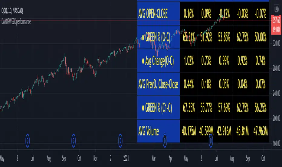
DAYOFWEEK performance1 -Objective
"What is the ''best'' day to trade .. Monday, Tuesday...."
This script aims to determine if there are different results depending on the day of the week.
The way it works is by dividing data by day of the week (Monday, Tuesday, Wednesday ... ) and perform calculations for each day of the week.
1 - Objective
2 - Features
3 - How to use (Examples)
4 - Inputs
5 - Limitations
6 - Notes
7 - Final Tooughs
2 - Features
AVG OPEN-CLOSE
Calculate de Percentage change from day open to close
Green % (O-C)
Percentage of days green (open to close)
Average Change
Absolute day change (O-C)
AVG PrevD. Close-Close
Percentage change from the previous day close to the day of the week close
(Example: Monday (C-C) = Friday Close to Monday close
Tuesday (C-C) = Monday C. to Tuesday C.
Green % (C1-C)
Percentage of days green (open to close)
AVG Volume
Day of the week Average Volume
Notes:
*Mon(Nº) - Nº = Number days is currently calculated
Example: Monday (12) calculation based on the last 12 Mondays. Note: Discrepancies in numbers example Monday (12) - Friday (11) depend on the initial/end date or the market was closed (Holidays).
3 - How to use (Examples)
For the following example, NASDAQ:AAPL from 1 Jan 21 to 1 Jul 21 the results are following.
The highest probability of a Close being higher than the Open is Monday with 52.17 % and the Lowest Tuesday with 38.46 %. Meaning that there's a higher chance (for NASDAQ:AAPL ) of closing at a higher value on Monday while the highest chance of closing is lower is Tuesday. With an average gain on Tuesday of 0.21%
Long - The best day to buy (long) at open (on average) is Monday with a 52.2% probability of closing higher
Short - The best day to sell (short) at open (on average) is Tuesday with a 38.5% probability of closing higher (better chance of closing lower)
Since the values change from ticker to ticker, there is a substantial change in the percentages and days of the week. For example let's compare the previous example ( NASDAQ:AAPL ) to NYSE:GM (same settings)
For the same period, there is a substantial difference where there is a 62.5% probability Friday to close higher than the open, while Tuesday there is only a 28% probability.
With an average gain of 0.59% on Friday and an average loss of -0.34%
Also, the size of the table (number of days ) depends if the ticker is traded or not on that day as an example COINBASE:BTCUSD
4 - Inputs
DATE RANGE
Initial Date - Date from which the script will start the calculation.
End Date - Date to which the script will calculate.
TABLE SETTINGS
Text Color - Color of the displayed text
Cell Color - Background color of table cells
Header Color - Color of the column and row names
Table Location - Change the position where the table is located.
Table Size - Changes text size and by consequence the size of the table
5 - LIMITATIONS
The code determines average values based on the stored data, therefore, the range (Initial data) is limited to the first bar time.
As a consequence the lower the timeframe the shorter the initial date can be and fewer weeks can be calculated. To warn about this limitation there's a warning text that appears in case the initial date exceeds the bar limit.
Example with initial date 1 Jan 2021 and end date 18 Jul 2021 in 5m and 10 m timeframe:
6 - Notes and Disclosers
The script can be moved around to a new pane if need. -> Object Tree > Right Click Script > Move To > New pane
The code has not been tested in higher subscriptions tiers that allow for more bars and as a consequence more data, but as far I can tell, it should work without problems and should be in fact better at lower timeframes since it allows more weeks.
The values displayed represent previous data and at no point is guaranteed future values
7 - Final Tooughs
This script was quite fun to work on since it analysis behavioral patterns (since from an abstract point a Tuesday is no different than a Thursday), but after analyzing multiple tickers there are some days that tend to close higher than the open.
PS: If you find any mistake ex: code/misspelling please comment.
ค้นหาในสคริปต์สำหรับ "12月4号是什么星座"
Phoenix Ascending 2.201Hi Everyone!
It's time to make this indicator public to relieve myself of replying to requests for access. There has been an update to this indicator; in which a Stochastic RSI was added to this indicator. Please follow the directions to SETUP the indicator in the SETUP VIDEO provided below.
Phoenix Ascending 2.201 and Bollinger Bands Setup Video.
The following are BASIC rules for the Phoenix 2.201 Indicator. More advanced rules and the requirements for those rules can be found in my publications in my public profile. Unfortunately, I do not have organized videos created on how to use this indicator in full but will be available in the future.
IMPORTANT: The BASIC rules below are beneficial but these are NOT all the rules. More rules and requirements for those rules will be available in the future.
RULE NO. 1
We PREFER the Blue LSMA to be at 80% or higher for SAFE EXIT (SHORT) bets.
We PREFER the Blue LSMA to be at 20% or lower for SAFE ENTRY (LONG) bets.
Rule No. 2
ANY time the red line is approaching a green line that’s moving UPWARD,
Be prepared to make an ENTRY (LONG) when the red line is about to touch the green line that’s moving upward.
One can look at a lower time frame to get a better idea of how much longer you may have
To wait for the red line to touch the green line. In many cases, you may make ENTRY (LONG)
Just before the red line actually touches the green line that’s moving up in that higher time frame
You were initially using as your COMPASS. I currently have the 1-Month TF as a compass for EURUSD.
Rule No. 3
ANY time the red line is approaching a green line that’s moving DOWNWARD,
Be prepared to make an EXIT (SHORT) when the red line is about to touch the green line that’s moving downward.
One can look at a lower time frame to get a better idea of how much longer you may have
To wait for the red line to touch the green line. In many cases, you may make your EXIT (SHORT)
Just before the red line actually touches the green line that’s moving downward in that higher time frame
You were initially using as your COMPASS. I currently have the 1-Month TF as a compass for EURUSD.
Rule No. 4
The Green Line and/or Ghost Line can often help one determine when an upward or downward move in a particular time frame
Is nearly exhausted and about to reverse.
Example for Upside Exhaustion about to reverse to the Downside:
When the Green Line and/or Ghost line is at 80% level or higher, this is a good indicator to inform
Us the current upside move may be approaching exhaustion. You can look at a higher time frame to try to gain
More insight as to whether this will only be a brief dip down in the lower time frame IF the higher time frame you
Went to reveals there is a lot more room remaining for the Green and/or Ghost Lines to reach the 80% or higher level.
Example for Downside Exhaustion about to reverse to the Upside:
When the Green Line and/or Ghost line is at 20% level or lower, this is a good indicator to inform
Us the current downside move may be approaching exhaustion. You can look at a higher time frame to try to gain
More insight as to whether this will only be a brief dip up in the lower time frame IF the higher time frame you
Went to reveals there is a lot more room remaining for the Green and/or Ghost Lines to reach the 20% or lower level.
Rule No. 5
The same rules you see in Rule No. 4 also apply to the Stochastic RSI. Keep in mind I changed the colors of the
Stochastic RSI to the following: Red default changed to Purple and Blue changed changed to Black to avoid confusing
Them with the lines in Godmode.
When the Stochastic RSI is at 80% or higher level, we need to be on guard for a reversal to the downside.
When the Stochastic RSI is at 20% or lower level, we need to be on guard for a reversal to the upside.
EXTREMELY IMPORTANT to apply these rules in GROUPS OF TIME FRAMES.
"TYPES" OF TIME FRAME GROUP TRADING SIGNALS
Scalping Group Signals: Signals provided for this group involve analyzing the following two groups of time frames. Short Term Group as a compass and Scalping Group for confirmation and more precise entry/exit.
Scalping Group: 6min. 12min. 23min & 45min.
Short Term Group: 90min. 3hr. 6hr. & 12hr.
Short Term Group Signals: Signals provided for this group involve analyzing the following two groups of time frames. NearTerm Group as a compass and Short Term Group for confirmation and more precise entry/exit.
Short Term Group: 90min. 3hr. 6hr. & 12hr.
Near Term Group: 24hr. 2-Day, 3-Day & 4-Day
Near Term Group Signals: Signals provided for this group involve analyzing the following two groups of time frames. Mid Term Group as a compass and Near Term Group for confirmation and more precise entry/exit.
Near Term Group: 24hr. 2-Day, 3-Day & 4-Day
Mid Term Group: 3-Day, 6-Day, 9-Day & 12-Day
Mid Term Group Signals: Signals provided for this group involve analyzing the following two groups of time frames. Long Term Group as a compass and Mid Term Group for confirmation and more precise entry/exit.
Mid Term Group: 3-Day, 6-Day, 9-Day & 12-Day
Long Term Group: 1-Week, 2-Week, 3-Week & 4-Week
Long Term Group Signals: Signals provided for this group involve analyzing the following two groups of time frames. Macro Term Group as a compass and Long Term Group for confirmation and more precise entry/exit.
Long Term Group: 1-Week, 2-Week, 3-Week & 4-Week
Macro Term Group: 1-Month, 2-Month, 3-Month & 4-Month
Macro Term Group Signals: Signals provided for this group involve analyzing the following two groups of time frames. Macro Term Group as a compass and Long Term Group for confirmation and more precise entry/exit.
Macro Term Group: 1-Month, 2-Month, 3-Month & 4-Month
Super Macro Group: 3-Month , 6-Month, 12-Month & 24-Month

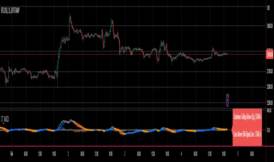
Reverse MACD IndicatorIntroducing the reverse MACD Indicator.
This is my Pinescript implementation of the reverse MACD indicator.
Much respect to Mr Johnny Dough the original creator of this idea.
Feel free to reuse this script, drop me a note below if you find this useful.
Investopedia defines the MACD as a trend-following momentum indicator that shows the relationship between two moving averages of a security’s price.
The MACD is calculated by subtracting the 26-period Exponential Moving Average ( EMA ) from the 12-period EMA .
The result of that calculation is the MACD line.
A nine-day EMA of the MACD called the "signal line," is then plotted on top of the MACD line, which can function as a trigger for buy and sell signals.
Traders may buy the security when the MACD crosses above its signal line and sell—or short—the security when the MACD crosses below the signal line.
Moving Average Convergence Divergence ( MACD ) indicators can be interpreted in several ways, but the more common methods are crossovers, divergences, and rapid rises/falls.
MACD triggers technical signals when it crosses above (to buy) or below (to sell) its signal line.
The speed of crossovers is also taken as a signal of a market is overbought or oversold.
MACD helps investors understand whether the bullish or bearish movement in the price is strengthening or weakening.
The MACD has a positive value (shown as the red line on the price chart ) whenever the 12-period EMA ( indicated by the blue line on the price chart) is above the 26-period EMA (the red line in the price chart) and a negative value when the 12-period EMA is below the 26-period EMA .
The more distant the MACD is above or below its baseline indicates that the distance between the two EMAs is growing.
The baseline here is the white line.
The Reverse function of the MACD provides value by letting the user know the specific price needed to expect a MACD cross over in the opposite direction.
This function can be used to designate risk parameters for a potential trade if using the MACD as their source of edge, letting the user know exactly where and how much their risk is for a potential trade which can be used to design an effective trading plan.
Percentage Volume Oscillator (PVO)The Percentage Volume Oscillator (PVO) is a momentum oscillator for volume. The PVO measures the difference between two volume-based moving averages as a percentage of the larger moving average. As with MACD and the Percentage Price Oscillator (PPO), it is shown with a signal line, a histogram and a centerline. The PVO is positive when the shorter volume EMA is above the longer volume EMA and negative when the shorter volume EMA is below. This indicator can be used to define the ups and downs for volume, which can then be used to confirm or refute other signals. Typically, a breakout or support break is validated when the PVO is rising or positive.
Generally speaking, volume is above average when the PVO is positive and below average when the PVO is negative. A negative and rising PVO indicates that volume levels are increasing. A positive and falling PVO indicates that volume levels are decreasing. Chartists can use this information to confirm or refute movements on the price chart.
Even though the PVO is based on a momentum oscillator formula, it is important to remember that moving averages lag. A 12-day EMA include 12 days of volume data, with newer data weighted more heavily. A 26-day EMA lags even more because it contains 26 days of data. This means that the PVO(12,26,9) can sometimes be out of sync with price action.
The Percentage Volume Oscillator (PVO) is a momentum indicator applied to volume. This oscillator can be quite choppy due to the fact that volume doesn't trend. Bullish and bearish divergences are not well suited for the PVO. Instead, chartists would be better off looking for signs of increasing volume with a move into positive territory and signs of decreasing volume with a move into negative territory. Increasing volume can validate a support or resistance break. Similarly, a surge or significant support break on low volume may be less robust. As with all technical indicators, it is important to use the Percentage Volume Oscillator (PVO) in conjunction with other aspects of technical analysis, such as chart patterns and momentum oscillators.

ETF / Stocks / Crypto - DCA Strategy v1Simple "benchmark" strategy for ETFs, Stocks and Crypto! Super-easy to implement for beginners, a DCA (dollar-cost-averaging) strategy means that you buy a fixed amount of an ETF / Stock / Crypto every several months. For instance, to DCA the S&P 500 (SPY), you could purchase $10,000 USD every 12 months, irrespective of the market price. Assuming the macro-economic conditions of the underlying country remain favourable, DCA strategies will result in capital gains over a period of many years, e.g. 10 years. DCA is the safest strategy that beginners can employ to make money in the markets, and all other types of strategies should be "benchmarked" against DCA; if your strategy cannot outperform DCA, then your strategy is useless.
Recommended Chart Settings:
Asset Class: ETF / Stocks / Crypto
Time Frame: H1 (Hourly) / D1 (Daily) / W1 (Weekly) / M1 (Monthly)
Necessary ETF Macro Conditions:
1. Country must have healthy demographics, good ratio of young > old
2. Country population must be increasing
3. Country must be experiencing price-inflation
Necessary Stock Conditions:
1. Growing revenue
2. Growing net income
3. Consistent net margins
4. Higher gross/net profit margin compared to its peers in the industry
5. Growing share holders equity
6. Current ratios > 1
7. Debt to equity ratio (compare to peers)
8. Debt servicing ratio < 30%
9. Wide economic moat
10. Products and services used daily, and will stay relevant for at least 1 decade
Necessary Crypto Conditions:
1. Honest founders
2. Competent technical co-founders
3. Fair or non-existent pre-mine
4. Solid marketing and PR
5. Legitimate use-cases / adoption
Default Robot Settings:
Contribution (USD): $10,000
Frequency (Months): 12
*Robot buys $10,000 worth of ETF, Stock, Crypto, regardless of the market price, every 12 months since its founding time.*
*Equity curve can be seen from the bottom panel*
Risk Warning:
This strategy is low-risk, however it assumes you have a long time horizon of at least 5 to 10 years. The longer your holding-period, the better your returns. The only thing the user has to keep-in-mind are the macro-economic conditions as stated above. If unsure, please stick to ETFs rather than buying individual stocks or cryptocurrencies.

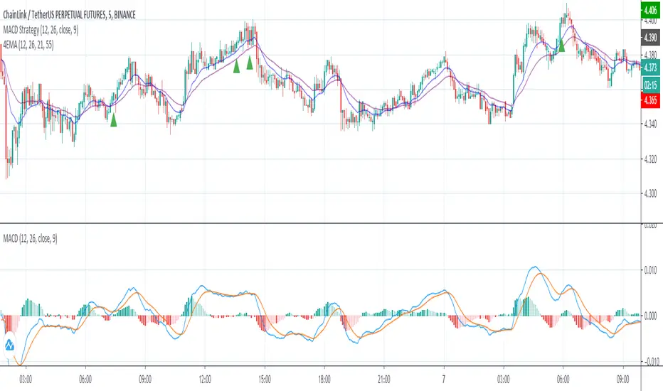
MACD StrategyThis script sends buy and sell signals as alerts to 3Commas (online software with trading bots in cryptocurreny)
It's based on 2 indicators:
- MACD
- 12 EMA and 26 EMA
When the 12 EMA and 26 EMA crossover, the MACD line crosses above 0. The goal here is to look for buy signals when the MACD and Signal are below 0, the histogram is positive, and there was or will be a 12 EMA and 26 EMA crossover.
I struggle with the following:
- There are multiple ways to use this as a crossover signal. I want to calculate the win rate of every posibility.
- What should be my take profit and my stoploss?
I think a 2:1 R/R,and a 60% win rate would make a great strategy! I could use some advice.
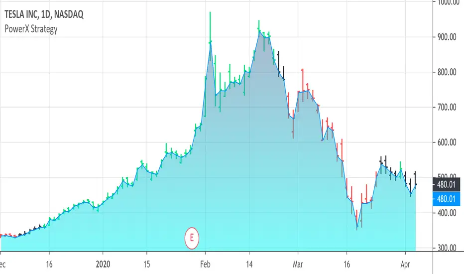
PowerX Strategy Bar Coloring [OFFICIAL VERSION]This script colors the bars according to the PowerX Strategy by Markus Heitkoetter:
The PowerX Strategy uses 3 indicators:
- RSI (7)
- Stochastics (14, 3, 3)
- MACD (12, 26 , 9)
The bars are colored GREEN if...
1.) The RSI (7) is above 50 AND
2.) The Stochastic (14, 3, 3) is above 50 AND
3.) The MACD (12, 26, 9) is above its Moving Average, i.e. MACD Histogram is positive.
The bars are colored RED if...
1.) The RSI (7) is below 50 AND
2.) The Stochastic (14, 3, 3) is below 50 AND
3.) The MACD (12, 26, 9) is below its Moving Average, i.e. MACD Histogram is negative.
If only 2 of these 3 conditions are met, then the bars are black (default color)
We highly recommend plotting the indicators mentioned above on your chart, too, so that you can see when bars are getting close to being "RED" or "GREEN", e.g. RSI is getting close to the 50 line.
Price Action and 3 EMAs Momentum plus Sessions FilterThis indicator plots on the chart the parameters and signals of the Price Action and 3 EMAs Momentum plus Sessions Filter Algorithmic Strategy. The strategy trades based on time-series (absolute) and relative momentum of price close, highs, lows and 3 EMAs.
I am still learning PS and therefore I have only been able to write the indicator up to the Signal generation. I plan to expand the indicator to Entry Signals as well as the full Strategy.
The strategy works best on EURUSD in the 15 minutes TF during London and New York sessions with 1 to 1 TP and SL of 30 pips with lots resulting in 3% risk of the account per trade. I have already written the full strategy in another language and platform and back tested it for ten years and it was profitable for 7 of the 10 years with average profit of 15% p.a which can be easily increased by increasing risk per trade. I have been trading it live in that platform for over two years and it is profitable.
Contributions from experienced PS coders in completing the Indicator as well as writing the Strategy and back testing it on Trading View will be appreciated.
STRATEGY AND INDICATOR PARAMETERS
Three periods of 12, 48 and 96 in the 15 min TF which are equivalent to 3, 12 and 24 hours i.e (15 min * period / 60 min) are the foundational inputs for all the parameters of the PA & 3 EMAs Momentum + SF Algo Strategy and its Indicator.
3 EMAs momentum parameters and conditions
• FastEMA = ema of 12 periods
• MedEMA = ema of 48 periods
• SlowEMA = ema of 96 periods
• All the EMAs analyse price close for up to 96 (15 min periods) equivalent to 24 hours
• There’s Upward EMA momentum if price close > FastEMA and FastEMA > MedEMA and MedEMA > SlowEMA
• There’s Downward EMA momentum if price close < FastEMA and FastEMA < MedEMA and MedEMA < SlowEMA
PA momentum parameters and conditions
• HH = Highest High of 48 periods from 1st closed bar before current bar
• LL = Lowest Low of 48 periods from 1st closed bar from current bar
• Previous HH = Highest High of 84 periods from 12th closed bar before current bar
• Previous LL = Lowest Low of 84 periods from 12th closed bar before current bar
• All the HH & LL and prevHH & prevLL are within the 96 periods from the 1st closed bar before current bar and therefore indicative of momentum during the past 24 hours
• There’s Upward PA momentum if price close > HH and HH > prevHH and LL > prevLL
• There’s Downward PA momentum if price close < LL and LL < prevLL and HH < prevHH
Signal conditions and Status (BuySignal, SellSignal or Neutral)
• The strategy generates Buy or Sell Signals if both 3 EMAs and PA momentum conditions are met for each direction and these occur during the London and New York sessions
• BuySignal if price close > FastEMA and FastEMA > MedEMA and MedEMA > SlowEMA and price close > HH and HH > prevHH and LL > prevLL and timeinrange (LDN&NY) else Neutral
• SellSignal if price close < FastEMA and FastEMA < MedEMA and MedEMA < SlowEMA and price close < LL and LL < prevLL and HH < prevHH and timeinrange (LDN&NY) else Neutral
Entry conditions and Status (EnterBuy, EnterSell or Neutral)(NOT CODED YET)
• ENTRY IS NOT AT THE SIGNAL BAR but at the current bar tick price retracement to FastEMA after the signal
• EnterBuy if current bar tick price <= FastEMA and current bar tick price > prevHH at the time of the Buy Signal
• EnterSell if current bar tick price >= FastEMA and current bar tick price > prevLL at the time of the Sell Signal

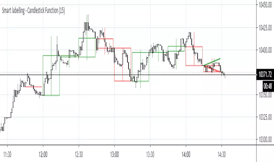
Smart labelling - Candlestick FunctionOftentimes a single look at the candlestick configuration happens to be enough to understand what is going on. The chandlestick function is an experiment in smart labelling that produces candles for various time frames, not only for the fixed 1m, 3m , 5m, 15m, etc. ones, and helps in decision-making when eye-balling the chart. This function generates up to 12 last candlesticks , which is generally more than enough.
Mind that since this is an experiment, the function does not cover all possible combinations. In some time frames the produced candles overlap. This is a todo item for those who are unterested. For instance, the current version covers the following TFs:
Chart - TF in the script
1m - 1-20,24,30,32
3m - 1-10
5m - 1-4,6,9,12,18,36
15m - 1-4,6,12
Tested chart TFs: 1m, 3m ,5m,15m. Tested securities: BTCUSD , EURUSD
[astropark] Power Tools Overlay//******************************************************************************
// Power Tools Overlay
// Inner Version 1.2.1 13/12/2018
// Developer: iDelphi
// Developer: astropark (Ichimoku Cloud), SMA EMA & Cross tools
//------------------------------------------------------------------------------
// 21/11/2018 Added EMA SMA WMA
// 21/11/2018 Added SMA-EMA EMA-WMA WMA-SMA (Thanks to mariobros1 for the idea of the Simultaneous MA)
// 21/11/2018 Added Bollinger Bands
// 21/11/2018 Added Ichimoku Cloud (Thanks to astropark for all the code of the Ichimoku Cloud)
// 23/11/2018 Show all the indicator as default
// 23/11/2018 Added a cross when single Moving Averages crossing (Thanks to astropark for the idea)
// 24/11/2018 Descriptions Fix
// 24/11/2018 Added Option to enable/disable all Moving Averages
// 10/12/2018 Added EMAs and Crosses
// 13/12/2018 indicator number fixes
//******************************************************************************

[Delphi] Power Tools OscillatorsFEATURES
- RSI
- Stochastic
//******************************************************************************
// Power Tools Oscillators
// Inner Version 1.0 04/12/2018
// Developer: iDelphi
//------------------------------------------------------------------------------
// 04/12/2018 Added RSI
// 04/12/2018 Added Stochastic
//******************************************************************************

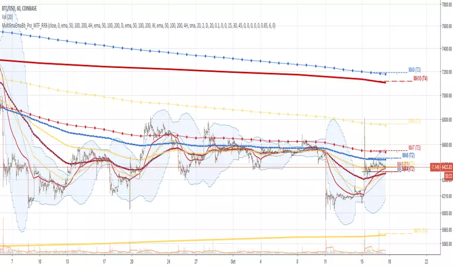
Multi SMA EMA WMA HMA BB (4x3 MAs Bollinger Bands) Pro MTF - RRBMulti SMA EMA WMA HMA 4x3 Moving Averages with Bollinger Bands Pro MTF by RagingRocketBull 2018
Version 1.0
This indicator shows multiple MAs of any type SMA EMA WMA HMA etc with BB and MTF support, can show MAs as dynamically moving levels.
There are 4 MA groups + 1 BB group. You can assign any type/timeframe combo to a group, for example:
- EMAs 50,100,200 x H1, H4, D1, W1 (4 TFs x 3 MAs x 1 type)
- EMAs 8,13,21,55,100,200 x M15, H1 (2 TFs x 6 MAs x 1 type)
- D1 EMAs and SMAs 12,26,50,100,200,400 (1 TF x 6 MAs x 2 types)
- H1 WMAs 7,77,231; H4 HMAs 50,100,200; D1 EMAs 144,169,233; W1 SMAs 50,100,200 (4 TFs x 3 MAs x 4 types)
- +1 extra MA type/timeframe for BB
compile time: 25-30 sec
full redraw time after parameter change in UI: 3 sec
There are several versions: Simple, MTF, Pro MTF, Advanced MTF and Ultimate MTF. This is the Pro MTF version. The Differences are listed below. All versions have BB
- Simple: you have 2 groups of MAs that can be assigned any type (5+5)
- MTF: +2 custom Timeframes for each group (2x5 MTF)
- Pro MTF: +4 custom Timeframes for each group (4x3 MTF), MA levels and show max bars back options
- Advanced MTF: +2 extra MAs/group (4x5 MTF), custom Ticker/Symbol, backreferences for type, TF and MA lengths in UI
- Ultimate MTF: +individual settings for each MA, custom Ticker/Symbols
Features:
- 4x3 = 12 MAs of any type including Hull Moving Average (HMA)
- 4x MTF groups with step line smoothing
- BB +1 extra TF/type for BB MAs
- 12 MA levels with adjustable group offsets, indents and shift
- show max bars back
- you can show/hide both groups of MAs/levels and individual MAs
Notes:
1. based on 3EmaBB, uses plot*, barssince and security functions
2. you can't set certain constants from input due to Pinescript limitations - change the code as needed, recompile and use as a private version
3. Levels = trackprice implementation
4. Show Max Bars Back = show_last implementation
5. uses timeframe textbox instead of input resolution to allow for 120 240 and other custom TFs. Also supports TFs in hours: 2H or H2
6. swma has a fixed length = 4, alma and linreg have additional offset and smoothing params
7. Smoothing is applied by default for visual aesthetics on MTF. To use exact ma mtf values (lines with stair stepping) - disable it
MTF Notes:
- uses simple timeframe textbox instead of input resolution dropdown to allow for 120, 240 and other custom TFs, also supports timeframes in H: 2H, H2
- Groups that are not assigned a Custom TF will use Current Timeframe (0).
- MTF will work for any MA type assigned to the group
- MTF works both ways: you can display a higher TF MA/BB on a lower TF or a lower TF MA/BB on a higher TF.
- MTF MA values are normally aligned at the boundary of their native timeframe. This produces stair stepping when a higher TF MA is viewed on a lower TF.
Therefore X Y Point Density/Smoothing is applied by default on MA MTF for visual aesthetics. Set both to 0 to disable and see exact ma mtf values (lines with stair stepping and original mtf alignment).
- Smoothing is disabled for BB MTF bands because fill doesn't work with smoothed MAs after duplicate values are replaced with na.
- MTF MA Value fluctuation is possible on the current bar due to default security lookahead
Smoothing:
- X,Y == 0 - X,Y smoothing disabled (stair stepping on high TFs)
- X == 0, Y > 0 - X,Y smoothing applied to all TFs
- Y == 0, X > 0 - X smoothing applied to all TFs < deltaX_max_tf, Y smoothing disabled
- X > 0, Y > 0 - Y smoothing applied to all TFs, then X smoothing applied to all TFs < deltaX_max_tf
X Smoothing with Y == 0 - shows only every deltaX-th point starting from the first bar.
X Smoothing with Y > 0 - shows only every deltaX-th point starting from the last shown Y point, essentially filling huge gaps remaining after Y Smoothing with points and preserving the curve's general shape
X Smoothing on high TFs with already scarce points produces weird curve shapes, it works best only on high density lower TFs
Y Smoothing reduces points on all TFs, removes adjacent points with prices within deltaY, while preserving the smaller curve details.
A combination of X,Y produces the most accurate smoothing. Higher delta value - larger range, more points removed.
Show Max Bars Back:
- can't set plot show_last from input -> implemented using a timenow based range check
- you can't delete/modify history once plotted, so essentially it just sets a start point for plotting (from num_bars bars back) that works only in realtime mode (not in replay)
Levels:
You can plot current MA value using plot trackprice=true or by checking Show Price Line in Style. Problem is:
- you can only change color (not the dashed line style, width), have both ma + price line (not just the line), and it's full screen wide
- you can't set plot trackprice from input => implemented using plotshape/plotchar with fixed text labels serving as levels
- there's no other way of creating a dynamic level: hline, plot, offset - nothing else works.
- you can't plot a text var - all text strings must be constants, so you can't change the style, width and text labels without recompiling.
- from input you can only adjust offset, indent and shift for each level group, and change color
- the dot below each level line is the exact MA value. If you want just the line swap plotshape with plotchar, recompile and save as your private version, adjust Y shift.
To speed up redraw times: reduce last_bars to ~2000, recompile and use as your own private version
Pinescript is a rudimentary language (should be called Painscript instead) that can basically only plot data. You can't do much else. Please see the code for tips and hints.
Certain things just can't be done or require shady workarounds and weeks of testing trying to resolve weird node.js compiler errors.
Feel free to learn from/reuse/change the code as needed and use as your own private version. See comments in code. Good Luck!
coinjin 정·역배열 대시보드 (Progress+Events)This script analyzes trend alignment using the 5 / 20 / 60 / 112 / 224 / 448 / 896 SMAs,
providing highly precise detection of bullish and bearish stack conditions,
and identifies 12 advanced trend-reversal signals through a multi-timeframe dashboard.
이 스크립트는 5 / 20 / 60 / 112 / 224 / 448 / 896 SMA 기준으로
정배열·역배열 상태를 매우 정교하게 분석하고,
12가지 고급 추세 전환 시그널을 자동 탐지하는 멀티타임프레임 대시보드입니다.

Scout Regiment - MACD# Scout Regiment - MACD Indicator
## English Documentation
### Overview
Scout Regiment - MACD is an advanced implementation of the Moving Average Convergence Divergence indicator with enhanced features including dual divergence detection (histogram and MACD line), customizable moving average types, multi-timeframe analysis, and sophisticated visual elements. This indicator provides traders with comprehensive momentum analysis and high-probability reversal signals.
### What is MACD?
MACD (Moving Average Convergence Divergence) is a trend-following momentum indicator that shows the relationship between two moving averages:
- **MACD Line**: Difference between fast and slow EMAs
- **Signal Line**: Moving average of the MACD line
- **Histogram**: Difference between MACD line and signal line
- **Purpose**: Identifies trend direction, momentum strength, and potential reversals
### Key Features
#### 1. **Enhanced MACD Display**
**Three Core Components:**
**MACD Line** (Default: Blue/Orange, 2px)
- Fast EMA (13) minus Slow EMA (34)
- Shows momentum direction
- Color changes based on position relative to signal line:
- Blue: Above signal line (bullish)
- Orange: Below signal line (bearish)
- Can be toggled on/off
**Signal Line** (Default: White/Blue with transparency, 2px)
- EMA (9) of the MACD line
- Serves as trigger line for crossover signals
- Color varies based on settings
- Essential for identifying entry/exit points
**Histogram** (Default: 4-color gradient, 4px columns)
- Difference between MACD and signal line
- Visual representation of momentum strength
- Advanced 4-color scheme:
- **Dark Green (#26A69A)**: Positive and increasing (strong bullish)
- **Light Green (#B2DFDB)**: Positive but decreasing (weakening bullish)
- **Dark Red (#FF5252)**: Negative and decreasing (strong bearish)
- **Light Red (#FFCDD2)**: Negative but increasing (weakening bearish)
- Histogram tells the "story" of momentum changes
#### 2. **Customizable Moving Average Types**
**Oscillator MA Type** (MACD Line calculation):
- **EMA** (Exponential) - Default, more responsive
- **SMA** (Simple) - Smoother, less responsive
**Signal Line MA Type**:
- **EMA** (Exponential) - Default, faster signals
- **SMA** (Simple) - Slower, fewer false signals
**Flexibility**: Mix and match for different trading styles
- EMA/EMA: Most responsive (day trading)
- SMA/SMA: Smoothest (swing trading)
- EMA/SMA or SMA/EMA: Balanced approaches
#### 3. **Multi-Timeframe Capability**
**Current Chart Period** (Default: Enabled)
- Uses current timeframe automatically
- Simplest option for most traders
**Custom Timeframe Selection**
- Calculate MACD on any timeframe
- Display higher timeframe MACD on lower timeframe charts
- Example: View 1H MACD on 15min chart
- **Use Case**: Align lower timeframe trades with higher timeframe momentum
#### 4. **Visual Enhancement Features**
**Golden Cross / Death Cross Markers**
- Circles mark crossover points
- Color matches MACD line color
- Clearly identifies entry/exit signals
- Can be toggled on/off
**Zero Line** (White, 2px solid)
- Reference for positive/negative momentum
- Critical level for trend identification
- MACD above zero = Bullish bias
- MACD below zero = Bearish bias
**Color Transitions**
- MACD line changes color at signal line crosses
- Histogram shows momentum acceleration/deceleration
- Provides early warning of trend changes
#### 5. **Dual Divergence Detection System**
This indicator features TWO separate divergence detection systems:
**A. Histogram Divergence Detection**
- **Purpose**: Earlier divergence signals (most sensitive)
- **Detects**: Regular bullish and bearish divergences
- **Label**: "H涨" (Histogram Up), "H跌" (Histogram Down)
- **Special Feature**: Same-sign requirement option
- Top divergence: Both histogram points must be positive
- Bottom divergence: Both histogram points must be negative
- Filters out less reliable divergences
**B. MACD Line Divergence Detection**
- **Purpose**: Stronger, more reliable divergences
- **Detects**: Regular bullish and bearish divergences
- **Label**: "M涨" (MACD Up), "M跌" (MACD Down)
- **Use**: Confirmation of histogram divergences or standalone
**Divergence Types Explained:**
**Regular Bullish Divergence (Yellow)**
- **Price**: Lower lows
- **Indicator**: Higher lows (histogram OR MACD line)
- **Signal**: Potential upward reversal
- **Best**: Near support levels, oversold conditions
- **Entry**: After price breaks above recent resistance
**Regular Bearish Divergence (Blue)**
- **Price**: Higher highs
- **Indicator**: Lower highs (histogram OR MACD line)
- **Signal**: Potential downward reversal
- **Best**: Near resistance levels, overbought conditions
- **Entry**: After price breaks below recent support
#### 6. **Advanced Divergence Parameters**
**Histogram Divergence Settings:**
- **Price Reference**: Wicks (default) or Bodies
- **Right Lookback**: Bars to right of pivot (default: 2)
- **Left Lookback**: Bars to left of pivot (default: 5)
- **Max Range**: Maximum bars between divergences (default: 60)
- **Min Range**: Minimum bars between divergences (default: 5)
- **Same Sign Requirement**: Ensures both histogram points have same sign
- **Show Regular Divergence**: Toggle display
- **Show Labels**: Toggle divergence labels
**MACD Line Divergence Settings:**
- **Price Reference**: Wicks (default) or Bodies
- **Right Lookback**: Bars to right of pivot (default: 1)
- **Left Lookback**: Bars to left of pivot (default: 5)
- **Max Range**: Maximum bars between divergences (default: 60)
- **Min Range**: Minimum bars between divergences (default: 5)
- **Show Regular Divergence**: Toggle display
- **Show Labels**: Toggle divergence labels
**Independent Control**: Adjust histogram and MACD line divergences separately
### Configuration Settings
#### MACD Basic Settings
- **Fast EMA Period**: Fast moving average length (default: 13)
- **Slow EMA Period**: Slow moving average length (default: 34)
- **Signal Line Period**: Signal line length (default: 9)
- **Use Current Chart Period**: Auto-adjust to current timeframe
- **Select Period**: Choose custom timeframe
- **Show MACD & Signal Lines**: Toggle lines display
- **Show Cross Markers**: Toggle golden/death cross dots
- **Show Histogram**: Toggle histogram display
- **Show Crossover Color Change**: Enable MACD line color change
- **Show Histogram Colors**: Enable 4-color histogram scheme
- **Oscillator MA Type**: Choose SMA or EMA for MACD
- **Signal Line MA Type**: Choose SMA or EMA for signal
#### Histogram Divergence Settings
- **Show Histogram Divergence**: Enable histogram divergence detection
- **Price Reference**: Wicks or Bodies for price comparison
- **Right/Left Lookback**: Pivot detection parameters
- **Max/Min Range**: Distance constraints between pivots
- **Show Regular Divergence**: Display histogram divergence lines
- **Show Labels**: Display histogram divergence labels
- **Require Same Sign**: Enforce histogram sign consistency
#### MACD Line Divergence Settings
- **Show MACD Line Divergence**: Enable MACD line divergence detection
- **Price Reference**: Wicks or Bodies for price comparison
- **Right/Left Lookback**: Pivot detection parameters
- **Max/Min Range**: Distance constraints between pivots
- **Show Regular Divergence**: Display MACD line divergence lines
- **Show Labels**: Display MACD line divergence labels
### How to Use
#### For Basic Trend Following
1. **Enable Core Components**
- MACD line, signal line, and histogram
- Enable cross markers
2. **Identify Trend**
- MACD above zero = Uptrend
- MACD below zero = Downtrend
3. **Watch for Crossovers**
- Golden cross (MACD crosses above signal) = Buy signal
- Death cross (MACD crosses below signal) = Sell signal
4. **Confirm with Histogram**
- Increasing histogram = Strengthening trend
- Decreasing histogram = Weakening trend
#### For Divergence Trading
1. **Enable Both Divergence Systems**
- Histogram divergence (early signals)
- MACD line divergence (confirmation)
2. **Wait for Divergence Signals**
- "H涨" or "H跌" = Early warning
- "M涨" or "M跌" = Confirmation
3. **Best Divergences**
- Both histogram AND MACD line showing divergence
- Divergence at key support/resistance levels
- Multiple divergences on same trend
4. **Entry Timing**
- Wait for price structure break
- Enter on pullback after confirmation
- Use MACD crossover as trigger
#### For Multi-Timeframe Analysis
1. **Set Higher Timeframe**
- Example: 4H MACD on 1H chart
- Uncheck "Use Current Chart Period"
- Select desired timeframe
2. **Identify Higher TF Trend**
- MACD position relative to zero
- MACD vs signal line relationship
3. **Trade with HTF Direction**
- Only take long signals if HTF MACD bullish
- Only take short signals if HTF MACD bearish
4. **Use Current TF for Entries**
- Higher TF for bias
- Current TF for precise timing
#### For Histogram Analysis
1. **Enable 4-Color Histogram**
- Watch color transitions
- Dark colors = Strong momentum
- Light colors = Weakening momentum
2. **Momentum Stages**
- Dark green → Light green = Bullish losing steam
- Light red → Dark red = Bearish gaining strength
3. **Trade Transitions**
- Light green to light red = Momentum shift (potential reversal)
- Entry on confirmation crossover
### Trading Strategies
#### Strategy 1: Classic MACD Crossover
**Setup:**
- Standard settings (13/34/9)
- Enable MACD, signal line, and cross markers
- Clear trend on higher timeframe
**Entry:**
- **Long**: Golden cross (circle marker) above zero line
- **Short**: Death cross (circle marker) below zero line
**Confirmation:**
- Histogram color supporting direction
- Volume increase helps
**Stop Loss:**
- Below recent swing low (long)
- Above recent swing high (short)
**Exit:**
- Opposite crossover
- MACD crosses zero line against position
**Best For:** Trend following, clear trending markets
#### Strategy 2: Zero Line Bounce
**Setup:**
- Enable all components
- Established trend (MACD staying one side of zero)
- Wait for pullback to zero line
**Entry:**
- **Long**: MACD touches zero from above, bounces up with golden cross
- **Short**: MACD touches zero from below, bounces down with death cross
**Confirmation:**
- Histogram color change
- Price at support/resistance
**Stop Loss:**
- Just beyond zero line (opposite side)
**Exit:**
- Target previous extreme
- Or opposite crossover
**Best For:** Trend continuation, strong markets
#### Strategy 3: Dual Divergence Confirmation
**Setup:**
- Enable both histogram and MACD line divergences
- Price at extreme (high/low)
- Wait for divergence signals
**Entry:**
- **Long**: Both "H涨" AND "M涨" labels appear
- **Short**: Both "H跌" AND "M跌" labels appear
**Confirmation:**
- Price breaks structure
- Volume increase
- Golden/death cross confirms
**Stop Loss:**
- Beyond divergence pivot point
**Exit:**
- MACD crosses zero line
- Or opposite divergence appears
**Best For:** Reversal trading, swing trading
#### Strategy 4: Histogram Color Transition
**Setup:**
- Enable 4-color histogram
- Focus on color changes
- Price in trend
**Entry:**
- **Long**: Light red → Light green transition + golden cross
- **Short**: Light green → Light red transition + death cross
**Rationale:**
- Light colors show momentum exhaustion
- Color flip = momentum shift
- Early entry before full trend reversal
**Stop Loss:**
- Recent swing point
**Exit:**
- Histogram color turns light against position
- Or at predetermined target
**Best For:** Scalping, day trading, early entries
#### Strategy 5: Multi-Timeframe Momentum
**Setup:**
- Display higher timeframe MACD (e.g., 4H on 1H chart)
- Current chart shows current momentum
- Higher TF shows overall bias
**Entry:**
- **Long**: HTF MACD above zero + current TF golden cross
- **Short**: HTF MACD below zero + current TF death cross
**Confirmation:**
- HTF histogram supporting direction
- Both timeframes aligned
**Stop Loss:**
- Based on current timeframe structure
**Exit:**
- Current TF opposite crossover
- Or HTF MACD momentum weakens
**Best For:** Swing trading, high-probability setups
#### Strategy 6: Histogram-Only Divergence Scout
**Setup:**
- Enable only histogram divergence
- Use "same sign requirement"
- Focus on early signals
**Entry:**
- **Long**: "H涨" label + price at support
- **Short**: "H跌" label + price at resistance
**Confirmation:**
- Wait for MACD/signal crossover
- Or price structure break
**Advantage:**
- Earliest divergence signals
- Get in before crowd
**Risk:**
- More false signals than MACD line divergence
- Requires strict confirmation
**Stop Loss:**
- Tight stop beyond entry bar
**Exit:**
- Quick targets (30-50% of expected move)
- Or trail stop
**Best For:** Active traders, scalpers seeking early entries
### Best Practices
#### MACD Period Selection
**Standard (13/34/9)** - Default
- Balanced for most markets
- Good for day trading and swing trading
- Widely used, works with general market psychology
**Faster (8/21/5 or 12/26/9)**
- More responsive
- More signals, more noise
- Best for: Scalping, volatile markets
- Risk: More false signals
**Slower (21/55/13)**
- Smoother signals
- Fewer but stronger signals
- Best for: Swing trading, position trading
- Benefit: Higher reliability
#### Histogram vs MACD Line Divergences
**Histogram Divergence:**
- ✅ Earlier signals
- ✅ Catch moves before others
- ❌ More false signals
- ❌ Requires confirmation
- **Best for**: Active traders, scalpers
**MACD Line Divergence:**
- ✅ More reliable
- ✅ Stronger divergences
- ❌ Later signals
- ❌ May miss early moves
- **Best for**: Swing traders, conservative traders
**Both Together:**
- ✅ Maximum confidence
- ✅ Histogram for alert, MACD for confirmation
- ✅ Highest probability setups
- **Best for**: All traders seeking quality over quantity
#### Same Sign Requirement Feature
**Enabled (Recommended):**
- Filters low-quality divergences
- Top divergence: Both histogram points positive
- Bottom divergence: Both histogram points negative
- Results in fewer but more reliable signals
**Disabled:**
- More divergence signals
- Includes zero-line crossing divergences
- Higher false signal rate
- Only for experienced traders
#### Price Reference: Wicks vs Bodies
**Wicks (Default):**
- Uses high/low prices
- Catches all extremes
- More divergences detected
- Best for: Most trading styles
**Bodies:**
- Uses open/close prices
- Filters out spike movements
- Fewer but cleaner divergences
- Best for: Noisy markets, crypto
#### Visual Settings Recommendations
**For Beginners:**
- Enable: MACD line, signal line, histogram
- Enable: Cross markers
- Enable: Histogram colors
- Disable: Both divergence systems initially
- Focus: Learn basic crossovers first
**For Intermediate:**
- All basic components
- Add: Histogram divergence only
- Use: Same sign requirement
- Focus: Early reversal signals
**For Advanced:**
- All components
- Both divergence systems
- Custom parameters per market
- Multi-timeframe analysis
- Focus: High-probability confluence setups
### Indicator Combinations
**With Moving Averages (EMAs):**
- EMAs (21/55/144) show trend
- MACD shows momentum
- Enter when both align
- Exit when MACD turns first
**With RSI:**
- RSI for overbought/oversold
- MACD for momentum confirmation
- Divergence on both = Extremely strong signal
- RSI + MACD divergence = High probability trade
**With Volume:**
- Volume confirms MACD signals
- Crossover + volume spike = Valid breakout
- Divergence + volume divergence = Strong reversal
**With Support/Resistance:**
- S/R levels for entry/exit targets
- MACD divergence at levels = Highest probability
- MACD crossover at level = Strong confirmation
**With Bias Indicator:**
- Bias shows price deviation from EMA
- MACD shows momentum
- Both diverging = Powerful reversal signal
- Bias extreme + MACD divergence = High conviction trade
**With OBV:**
- OBV shows volume trend
- MACD shows price momentum
- OBV + MACD divergence = Volume not supporting price
- Strong reversal indication
**With KSI (RSI/CCI):**
- KSI for oscillator extremes
- MACD for momentum direction
- KSI extreme + MACD divergence = Reversal likely
- All aligned = Maximum confidence
### Common MACD Patterns
1. **Bullish Cross Above Zero**: Strong uptrend continuation signal
2. **Bearish Cross Below Zero**: Strong downtrend continuation signal
3. **Zero Line Rejection**: Price respects zero as support/resistance
4. **Histogram Peak**: Momentum climax, watch for reversal
5. **Double Divergence**: Two divergences without reversal = Very strong signal when it finally reverses
6. **Histogram Convergence**: Histogram narrowing = Trend losing steam
7. **Signal Line Hug**: MACD stays close to signal = Consolidation, expect breakout
### Performance Tips
- Start with default settings (13/34/9 EMA/EMA)
- Test one divergence system at a time
- Use same sign requirement initially
- Enable cross markers for clear signals
- Adjust lookback parameters per market volatility
- Higher timeframe MACD more reliable than lower
- Combine histogram early signal with MACD line confirmation
- Don't trade every divergence - wait for best setups
### Alert Conditions
While not explicitly coded, you can set custom alerts on:
- MACD crossing above/below signal line
- MACD crossing above/below zero line
- Histogram crossing zero
- When divergence labels appear (using visual alerts)
---
## 中文说明文档
### 概述
Scout Regiment - MACD 是移动平均线收敛发散指标的高级实现版本,具有增强功能,包括双重背离检测(直方图和MACD线)、可自定义的移动平均类型、多时间框架分析和复杂的视觉元素。该指标为交易者提供全面的动量分析和高概率反转信号。
### 什么是MACD?
MACD(移动平均线收敛发散)是一个趋势跟随动量指标,显示两条移动平均线之间的关系:
- **MACD线**:快速和慢速EMA之间的差值
- **信号线**:MACD线的移动平均
- **直方图**:MACD线和信号线之间的差值
- **用途**:识别趋势方向、动量强度和潜在反转
### 核心功能
#### 1. **增强的MACD显示**
**三个核心组件:**
**MACD线**(默认:蓝色/橙色,2像素)
- 快速EMA(13)减去慢速EMA(34)
- 显示动量方向
- 根据相对于信号线的位置改变颜色:
- 蓝色:信号线上方(看涨)
- 橙色:信号线下方(看跌)
- 可开关显示
**信号线**(默认:白色/蓝色带透明度,2像素)
- MACD线的EMA(9)
- 作为交叉信号的触发线
- 颜色根据设置变化
- 识别进出场点的关键
**直方图**(默认:4色渐变,4像素柱)
- MACD和信号线之间的差值
- 动量强度的视觉表示
- 高级4色方案:
- **深绿色(#26A69A)**:正值且增加(强劲看涨)
- **浅绿色(#B2DFDB)**:正值但减少(看涨减弱)
- **深红色(#FF5252)**:负值且减少(强劲看跌)
- **浅红色(#FFCDD2)**:负值但增加(看跌减弱)
- 直方图讲述动量变化的"故事"
#### 2. **可自定义的移动平均类型**
**振荡器MA类型**(MACD线计算):
- **EMA**(指数)- 默认,反应更快
- **SMA**(简单)- 更平滑,反应较慢
**信号线MA类型**:
- **EMA**(指数)- 默认,更快信号
- **SMA**(简单)- 更慢,假信号更少
**灵活性**:混合搭配以适应不同交易风格
- EMA/EMA:最灵敏(日内交易)
- SMA/SMA:最平滑(波段交易)
- EMA/SMA或SMA/EMA:平衡方法
#### 3. **多时间框架功能**
**当前图表周期**(默认:启用)
- 自动使用当前时间框架
- 大多数交易者的最简单选项
**自定义时间框架选择**
- 在任何时间框架上计算MACD
- 在低时间框架图表上显示高时间框架MACD
- 示例:在15分钟图上查看1小时MACD
- **使用场景**:使低时间框架交易与高时间框架动量保持一致
#### 4. **视觉增强功能**
**金叉/死叉标记**
- 圆点标记交叉点
- 颜色与MACD线颜色匹配
- 清晰识别进出场信号
- 可开关
**零线**(白色,2像素实线)
- 正负动量的参考
- 趋势识别的关键水平
- MACD在零线上方 = 看涨偏向
- MACD在零线下方 = 看跌偏向
**颜色转换**
- MACD线在信号线交叉处改变颜色
- 直方图显示动量加速/减速
- 提供趋势变化的早期警告
#### 5. **双重背离检测系统**
该指标具有两个独立的背离检测系统:
**A. 直方图背离检测**
- **用途**:更早的背离信号(最敏感)
- **检测**:常规看涨和看跌背离
- **标签**:"H涨"(直方图上涨)、"H跌"(直方图下跌)
- **特殊功能**:同符号要求选项
- 顶背离:两个直方图点都必须为正
- 底背离:两个直方图点都必须为负
- 过滤不太可靠的背离
**B. MACD线背离检测**
- **用途**:更强、更可靠的背离
- **检测**:常规看涨和看跌背离
- **标签**:"M涨"(MACD上涨)、"M跌"(MACD下跌)
- **用途**:确认直方图背离或独立使用
**背离类型说明:**
**常规看涨背离(黄色)**
- **价格**:更低的低点
- **指标**:更高的低点(直方图或MACD线)
- **信号**:潜在向上反转
- **最佳**:在支撑水平附近、超卖状况
- **入场**:价格突破近期阻力后
**常规看跌背离(蓝色)**
- **价格**:更高的高点
- **指标**:更低的高点(直方图或MACD线)
- **信号**:潜在向下反转
- **最佳**:在阻力水平附近、超买状况
- **入场**:价格跌破近期支撑后
#### 6. **高级背离参数**
**直方图背离设置:**
- **价格参考**:影线(默认)或实体
- **右侧回溯**:枢轴点右侧K线数(默认:2)
- **左侧回溯**:枢轴点左侧K线数(默认:5)
- **最大范围**:背离之间最大K线数(默认:60)
- **最小范围**:背离之间最小K线数(默认:5)
- **同符号要求**:确保两个直方图点符号相同
- **显示常规背离**:切换显示
- **显示标签**:切换背离标签
**MACD线背离设置:**
- **价格参考**:影线(默认)或实体
- **右侧回溯**:枢轴点右侧K线数(默认:1)
- **左侧回溯**:枢轴点左侧K线数(默认:5)
- **最大范围**:背离之间最大K线数(默认:60)
- **最小范围**:背离之间最小K线数(默认:5)
- **显示常规背离**:切换显示
- **显示标签**:切换背离标签
**独立控制**:分别调整直方图和MACD线背离
### 配置设置
#### MACD基础设置
- **快速EMA周期**:快速移动平均长度(默认:13)
- **慢速EMA周期**:慢速移动平均长度(默认:34)
- **信号线周期**:信号线长度(默认:9)
- **使用当前图表周期**:自动调整到当前时间框架
- **选择周期**:选择自定义时间框架
- **显示MACD线和信号线**:切换线条显示
- **显示金叉死叉圆点标记**:切换金叉/死叉圆点
- **显示直方图**:切换直方图显示
- **显示穿越变化MACD线**:启用MACD线颜色变化
- **显示直方图颜色**:启用4色直方图方案
- **振荡器MA类型**:为MACD选择SMA或EMA
- **信号线MA类型**:为信号线选择SMA或EMA
#### 直方图背离设置
- **显示直方图背离信号**:启用直方图背离检测
- **价格参考**:影线或实体用于价格比较
- **右侧/左侧回溯**:枢轴检测参数
- **最大/最小范围**:枢轴之间的距离约束
- **显示直方图常规背离**:显示直方图背离线
- **显示直方图常规背离标签**:显示直方图背离标签
- **要求背离点柱状图同符号**:强制直方图符号一致性
#### MACD线背离设置
- **显示MACD线背离信号**:启用MACD线背离检测
- **价格参考**:影线或实体用于价格比较
- **右侧/左侧回溯**:枢轴检测参数
- **最大/最小范围**:枢轴之间的距离约束
- **显示线常规背离**:显示MACD线背离线
- **显示线常规背离标签**:显示MACD线背离标签
### 使用方法
#### 基础趋势跟随
1. **启用核心组件**
- MACD线、信号线和直方图
- 启用交叉标记
2. **识别趋势**
- MACD在零线上方 = 上升趋势
- MACD在零线下方 = 下降趋势
3. **观察交叉**
- 金叉(MACD向上穿越信号线)= 买入信号
- 死叉(MACD向下穿越信号线)= 卖出信号
4. **用直方图确认**
- 直方图增加 = 趋势加强
- 直方图减少 = 趋势减弱
#### 背离交易
1. **启用两个背离系统**
- 直方图背离(早期信号)
- MACD线背离(确认)
2. **等待背离信号**
- "H涨"或"H跌" = 早期警告
- "M涨"或"M跌" = 确认
3. **最佳背离**
- 直方图和MACD线都显示背离
- 在关键支撑/阻力水平的背离
- 同一趋势上多个背离
4. **入场时机**
- 等待价格结构突破
- 确认后回调时进入
- 使用MACD交叉作为触发
#### 多时间框架分析
1. **设置更高时间框架**
- 示例:在1小时图上显示4小时MACD
- 取消勾选"使用当前图表周期"
- 选择所需时间框架
2. **识别更高TF趋势**
- MACD相对于零线的位置
- MACD与信号线的关系
3. **顺HTF方向交易**
- 仅在HTF MACD看涨时接受多头信号
- 仅在HTF MACD看跌时接受空头信号
4. **使用当前TF入场**
- 更高TF确定偏向
- 当前TF精确定时
#### 直方图分析
1. **启用4色直方图**
- 观察颜色转换
- 深色 = 强动量
- 浅色 = 动量减弱
2. **动量阶段**
- 深绿色→浅绿色 = 看涨失去动力
- 浅红色→深红色 = 看跌获得力量
3. **交易转换**
- 浅绿色到浅红色 = 动量转变(潜在反转)
- 确认交叉时入场
### 交易策略
#### 策略1:经典MACD交叉
**设置:**
- 标准设置(13/34/9)
- 启用MACD、信号线和交叉标记
- 更高时间框架明确趋势
**入场:**
- **多头**:零线上方金叉(圆点标记)
- **空头**:零线下方死叉(圆点标记)
**确认:**
- 直方图颜色支持方向
- 成交量增加有帮助
**止损:**
- 近期波动低点之下(多头)
- 近期波动高点之上(空头)
**离场:**
- 相反交叉
- MACD反向穿越零线
**适合:**趋势跟随、明确趋势市场
#### 策略2:零线反弹
**设置:**
- 启用所有组件
- 已建立趋势(MACD保持在零线一侧)
- 等待回调至零线
**入场:**
- **多头**:MACD从上方触及零线,向上反弹并金叉
- **空头**:MACD从下方触及零线,向下反弹并死叉
**确认:**
- 直方图颜色变化
- 价格在支撑/阻力位
**止损:**
- 零线对面一侧
**离场:**
- 目标前一极值
- 或相反交叉
**适合:**趋势延续、强势市场
#### 策略3:双重背离确认
**设置:**
- 启用直方图和MACD线背离
- 价格在极值(高点/低点)
- 等待背离信号
**入场:**
- **多头**:"H涨"和"M涨"标签都出现
- **空头**:"H跌"和"M跌"标签都出现
**确认:**
- 价格突破结构
- 成交量增加
- 金叉/死叉确认
**止损:**
- 背离枢轴点之外
**离场:**
- MACD穿越零线
- 或出现相反背离
**适合:**反转交易、波段交易
#### 策略4:直方图颜色转换
**设置:**
- 启用4色直方图
- 关注颜色变化
- 价格处于趋势
**入场:**
- **多头**:浅红色→浅绿色转换 + 金叉
- **空头**:浅绿色→浅红色转换 + 死叉
**原理:**
- 浅色显示动量衰竭
- 颜色翻转 = 动量转变
- 完全趋势反转前的早期入场
**止损:**
- 近期波动点
**离场:**
- 直方图颜色变为反向浅色
- 或预定目标
**适合:**剥头皮、日内交易、早期入场
#### 策略5:多时间框架动量
**设置:**
- 显示更高时间框架MACD(例如,在1小时图上显示4小时)
- 当前图表显示当前动量
- 更高TF显示整体偏向
**入场:**
- **多头**:HTF MACD在零线上方 + 当前TF金叉
- **空头**:HTF MACD在零线下方 + 当前TF死叉
**确认:**
- HTF直方图支持方向
- 两个时间框架对齐
**止损:**
- 基于当前时间框架结构
**离场:**
- 当前TF相反交叉
- 或HTF MACD动量减弱
**适合:**波段交易、高概率设置
#### 策略6:仅直方图背离侦察
**设置:**
- 仅启用直方图背离
- 使用"同符号要求"
- 关注早期信号
**入场:**
- **多头**:"H涨"标签 + 价格在支撑位
- **空头**:"H跌"标签 + 价格在阻力位
**确认:**
- 等待MACD/信号线交叉
- 或价格结构突破
**优势:**
- 最早的背离信号
- 在大众之前进入
**风险:**
- 比MACD线背离假信号更多
- 需要严格确认
**止损:**
- 入场K线之外紧密止损
**离场:**
- 快速目标(预期波动的30-50%)
- 或移动止损
**适合:**活跃交易者、寻求早期入场的剥头皮交易者
### 最佳实践
#### MACD周期选择
**标准(13/34/9)** - 默认
- 大多数市场的平衡
- 适合日内交易和波段交易
- 广泛使用,符合一般市场心理
**更快(8/21/5或12/26/9)**
- 更灵敏
- 更多信号,更多噪音
- 最适合:剥头皮、波动市场
- 风险:更多假信号
**更慢(21/55/13)**
- 更平滑的信号
- 信号较少但更强
- 最适合:波段交易、仓位交易
- 优势:更高可靠性
#### 直方图vs MACD线背离
**直方图背离:**
- ✅ 更早信号
- ✅ 在其他人之前捕捉波动
- ❌ 更多假信号
- ❌ 需要确认
- **最适合**:活跃交易者、剥头皮交易者
**MACD线背离:**
- ✅ 更可靠
- ✅ 更强的背离
- ❌ 信号较晚
- ❌ 可能错过早期波动
- **最适合**:波段交易者、保守交易者
**两者结合:**
- ✅ 最大信心
- ✅ 直方图警报,MACD确认
- ✅ 最高概率设置
- **最适合**:所有寻求质量而非数量的交易者
#### 同符号要求功能
**启用(推荐):**
- 过滤低质量背离
- 顶背离:两个直方图点都为正
- 底背离:两个直方图点都为负
- 产生更少但更可靠的信号
**禁用:**
- 更多背离信号
- 包括零线穿越背离
- 假信号率更高
- 仅适合有经验的交易者
#### 价格参考:影线vs实体
**影线(默认):**
- 使用最高/最低价
- 捕捉所有极值
- 检测到更多背离
- 最适合:大多数交易风格
**实体:**
- 使用开盘/收盘价
- 过滤突刺波动
- 背离更少但更干净
- 最适合:噪音市场、加密货币
#### 视觉设置建议
**新手:**
- 启用:MACD线、信号线、直方图
- 启用:交叉标记
- 启用:直方图颜色
- 禁用:初始禁用两个背离系统
- 重点:先学习基本交叉
**中级:**
- 所有基本组件
- 添加:仅直方图背离
- 使用:同符号要求
- 重点:早期反转信号
**高级:**
- 所有组件
- 两个背离系统
- 每个市场自定义参数
- 多时间框架分析
- 重点:高概率汇合设置
### 指标组合
**与移动平均线(EMA)配合:**
- EMA(21/55/144)显示趋势
- MACD显示动量
- 两者一致时进入
- MACD先转向时退出
**与RSI配合:**
- RSI用于超买超卖
- MACD用于动量确认
- 两者都背离 = 极强信号
- RSI + MACD背离 = 高概率交易
**与成交量配合:**
- 成交量确认MACD信号
- 交叉 + 成交量激增 = 有效突破
- 背离 + 成交量背离 = 强反转
**与支撑/阻力配合:**
- 支撑阻力水平用于进出目标
- 水平处的MACD背离 = 最高概率
- 水平处的MACD交叉 = 强确认
**与Bias指标配合:**
- Bias显示价格相对EMA的偏离
- MACD显示动量
- 两者都背离 = 强大反转信号
- Bias极值 + MACD背离 = 高信念交易
**与OBV配合:**
- OBV显示成交量趋势
- MACD显示价格动量
- OBV + MACD背离 = 成交量不支持价格
- 强反转迹象
**与KSI(RSI/CCI)配合:**
- KSI用于振荡器极值
- MACD用于动量方向
- KSI极值 + MACD背离 = 可能反转
- 全部对齐 = 最大信心
### 常见MACD形态
1. **零线上方看涨交叉**:强上升趋势延续信号
2. **零线下方看跌交叉**:强下降趋势延续信号
3. **零线拒绝**:价格将零线作为支撑/阻力
4. **直方图峰值**:动量高潮,注意反转
5. **双重背离**:两次背离未反转 = 最终反转时非常强
6. **直方图收敛**:直方图变窄 = 趋势失去动力
7. **信号线紧贴**:MACD紧贴信号线 = 盘整,预期突破
### 性能提示
- 从默认设置开始(13/34/9 EMA/EMA)
- 一次测试一个背离系统
- 初始使用同符号要求
- 启用交叉标记以获得清晰信号
- 根据市场波动性调整回溯参数
- 更高时间框架MACD比更低的更可靠
- 结合直方图早期信号与MACD线确认
- 不要交易每个背离 - 等待最佳设置
### 警报条件
虽然没有明确编码,但您可以设置自定义警报:
- MACD向上/向下穿越信号线
- MACD向上/向下穿越零线
- 直方图穿越零线
- 背离标签出现时(使用视觉警报)
---
## Technical Support
For questions or issues, please refer to the TradingView community or contact the indicator creator.
## 技术支持
如有问题,请参考TradingView社区或联系指标创建者。

Scout Regiment - D17# Scout Regiment - D17 Indicator
## English Documentation
### Overview
Scout Regiment - D17 is a comprehensive TradingView indicator that combines multiple technical analysis tools into one powerful overlay indicator. It provides traders with market structure analysis, divergence detection, volume profiling, smart money concepts, and session analysis.
### Key Features
#### 1. **EMA (Exponential Moving Averages)**
- **Purpose**: Trend identification and dynamic support/resistance levels
- **Configuration**: 13 customizable EMAs with adjustable periods
- **Default Active EMAs**: EMA 3 (21), EMA 5 (55), EMA 7 (144), EMA 8 (233)
- **Uses**: Identify trend direction, entry/exit points, and trend strength
- **Color Coding**: Different colors for easy visual distinction
#### 2. **TFMA (Timeframe Moving Averages)**
- **Purpose**: Multi-timeframe trend analysis
- **Features**:
- 3 EMAs on higher timeframes
- Dynamic labels showing trend direction
- Price difference percentage display
- Customizable timeframe settings
- **Default Settings**: 21-period timeframe with lengths 55, 144, and 233
- **Benefits**: Align trades with higher timeframe trends
#### 3. **DFMA (Daily Frame Moving Averages)**
- **Purpose**: Daily timeframe perspective on any chart
- **Features**: Similar to TFMA but specifically for daily analysis
- **Default Timeframe**: 1D (Daily)
- **Use Case**: Long-term trend confirmation and positioning
#### 4. **PMA (Price Moving Averages)**
- **Purpose**: Price channel analysis with filled areas
- **Configuration**: 7 customizable moving averages with fill zones
- **Default Lengths**: 12, 144, 169, 288, 338, 576, 676
- **Visual**: Color-filled zones between selected MAs for channel trading
#### 5. **VWAP (Volume Weighted Average Price)**
- **Purpose**: Institutional trading levels and fair value
- **Features**:
- Multiple anchor periods (Session, Week, Month, Quarter, Year, etc.)
- Standard deviation bands
- Corporate event anchoring (Earnings, Dividends, Splits)
- **Use Case**: Identify institutional support/resistance and mean reversion opportunities
#### 6. **Divergence Detector**
- **Purpose**: Identify potential trend reversals
- **Supported Indicators**: MACD, MACD Histogram, RSI, Stochastic, CCI, Williams %R, Bias, Momentum, OBV, SOBV, VWmacd, CMF, MFI, and external indicators
- **Divergence Types**:
- Regular Bullish/Bearish
- Hidden Bullish/Bearish
- **Features**:
- Automatic divergence line drawing
- Customizable detection parameters
- Color-coded alerts
#### 7. **Volume Profile & Node Detection**
- **Purpose**: Identify key price levels based on volume distribution
- **Features**:
- Volume Profile with POC (Point of Control)
- Value Area High (VAH) and Value Area Low (VAL)
- Peak and trough volume node detection
- Highest/lowest volume node highlighting
- **Lookback**: Configurable (default 377 bars)
- **Use Case**: Identify support/resistance zones and liquidity areas
#### 8. **Smart Money Concepts**
- **Purpose**: Track institutional trading patterns
- **Features**:
- Market Structure (BOS - Break of Structure, CHoCH - Change of Character)
- Internal and Swing structures
- Strong/Weak Highs and Lows
- Equal Highs/Lows detection
- Fair Value Gaps (FVG)
- **Modes**: Historical or Present (latest only)
- **Use Case**: Trade with institutional flow
#### 9. **Trading Sessions**
- **Purpose**: Analyze market behavior during different global sessions
- **Available Sessions**:
- Asian Session
- Sydney, Tokyo, Shanghai, Hong Kong
- European Session
- London, New York, NYSE
- **Features**:
- Session boxes with high/low visualization
- Real-time countdown timers
- Volume and price change tracking
- Information table with session statistics
- **Customization**: Choose which sessions to display, colors, and box styles
### How to Use
#### For Trend Following:
1. Enable EMAs 3, 5, 7, and 8
2. Use TFMA for higher timeframe confirmation
3. Look for price above/below key EMAs for trend direction
4. Use VWAP as additional confirmation
#### For Reversal Trading:
1. Enable Divergence Detector with MACD Histogram and Bias
2. Look for divergences at key support/resistance levels
3. Confirm with Smart Money CHoCH signals
4. Use Volume Profile nodes as entry/exit targets
#### For Intraday Trading:
1. Enable Trading Sessions
2. Focus on high-volume sessions (London, New York overlap)
3. Use session highs/lows as support/resistance
4. Trade Fair Value Gaps during active sessions
#### For Swing Trading:
1. Use DFMA for daily trend
2. Enable PMA for channel identification
3. Look for price reactions at volume profile value areas
4. Confirm with swing structure breaks
### Best Practices
1. **Don't Overcrowd**: Enable only the components you need for your strategy
2. **Multi-Timeframe Analysis**: Always check higher timeframe TFMA/DFMA
3. **Confluence**: Look for multiple signals confirming the same direction
4. **Volume Confirmation**: Use Volume Profile to validate price action
5. **Session Awareness**: Be aware of which session is active for volatility expectations
### Performance Optimization
- Disable unused features to improve chart loading speed
- Use "Present Mode" for Smart Money Concepts if historical data isn't needed
- Reduce Volume Profile lookback period on slower devices
### Alerts
The indicator includes alert conditions for:
- All divergence types (8 conditions)
- Smart Money structure breaks (8 conditions)
- Equal highs/lows detection
- Fair Value Gaps formation
---
## 中文说明文档
### 概述
Scout Regiment - D17 是一款综合性TradingView指标,将多个技术分析工具整合到一个强大的叠加指标中。它为交易者提供市场结构分析、背离检测、成交量分析、聪明钱概念和时区分析。
### 核心功能
#### 1. **EMA(指数移动平均线)**
- **用途**:趋势识别和动态支撑阻力位
- **配置**:13条可自定义周期的EMA
- **默认启用**:EMA 3(21)、EMA 5(55)、EMA 7(144)、EMA 8(233)
- **应用**:识别趋势方向、进出场点位和趋势强度
- **颜色编码**:不同颜色便于视觉区分
#### 2. **TFMA(时间框架移动平均线)**
- **用途**:多时间框架趋势分析
- **特点**:
- 3条更高时间框架的EMA
- 显示趋势方向的动态标签
- 价格差异百分比显示
- 可自定义时间框架设置
- **默认设置**:21周期时间框架,长度为55、144和233
- **优势**:使交易与更高时间框架趋势保持一致
#### 3. **DFMA(日线框架移动平均线)**
- **用途**:在任何图表上提供日线时间框架视角
- **特点**:与TFMA类似,但专门用于日线分析
- **默认时间框架**:1D(日线)
- **使用场景**:长期趋势确认和定位
#### 4. **PMA(价格移动平均线)**
- **用途**:价格通道分析与填充区域
- **配置**:7条可自定义的移动平均线,带填充区域
- **默认长度**:12、144、169、288、338、576、676
- **视觉效果**:选定MA之间的彩色填充区域,用于通道交易
#### 5. **VWAP(成交量加权平均价格)**
- **用途**:机构交易水平和公允价值
- **特点**:
- 多个锚定周期(交易日、周、月、季度、年等)
- 标准差波段
- 企业事件锚定(财报、分红、拆股)
- **使用场景**:识别机构支撑阻力和均值回归机会
#### 6. **背离检测器**
- **用途**:识别潜在趋势反转
- **支持指标**:MACD、MACD柱状图、RSI、随机指标、CCI、威廉指标、乖离率、动量、OBV、SOBV、VWmacd、CMF、MFI及外部指标
- **背离类型**:
- 常规看涨/看跌背离
- 隐藏看涨/看跌背离
- **特点**:
- 自动绘制背离连线
- 可自定义检测参数
- 颜色编码警报
#### 7. **成交量分布与节点检测**
- **用途**:基于成交量分布识别关键价格水平
- **特点**:
- 成交量分布图与POC(控制点)
- 价值区域高点(VAH)和低点(VAL)
- 峰值和低谷成交量节点检测
- 最高/最低成交量节点突出显示
- **回溯期**:可配置(默认377根K线)
- **使用场景**:识别支撑阻力区域和流动性区域
#### 8. **聪明钱概念**
- **用途**:追踪机构交易模式
- **特点**:
- 市场结构(BOS-突破结构、CHoCH-结构转变)
- 内部和摆动结构
- 强/弱高低点
- 等高/等低检测
- 公允价值缺口(FVG)
- **模式**:历史模式或当前模式(仅最新)
- **使用场景**:跟随机构资金流动交易
#### 9. **交易时区**
- **用途**:分析不同全球时段的市场行为
- **可用时段**:
- 亚洲时段
- 悉尼、东京、上海、香港
- 欧洲时段
- 伦敦、纽约、纽交所
- **特点**:
- 时段方框显示高低点
- 实时倒计时
- 成交量和价格变化追踪
- 时段统计信息表格
- **自定义**:选择显示哪些时段、颜色和方框样式
### 使用方法
#### 趋势跟随策略:
1. 启用EMA 3、5、7和8
2. 使用TFMA进行更高时间框架确认
3. 观察价格在关键EMA上方/下方确定趋势方向
4. 使用VWAP作为额外确认
#### 反转交易策略:
1. 启用背离检测器(MACD柱状图和乖离率)
2. 在关键支撑阻力位寻找背离
3. 用聪明钱CHoCH信号确认
4. 使用成交量分布节点作为进出场目标
#### 日内交易策略:
1. 启用交易时区
2. 关注高成交量时段(伦敦、纽约重叠时段)
3. 使用时段高低点作为支撑阻力
4. 在活跃时段交易公允价值缺口
#### 波段交易策略:
1. 使用DFMA确定日线趋势
2. 启用PMA识别通道
3. 观察价格在成交量分布价值区域的反应
4. 用摆动结构突破确认
### 最佳实践
1. **避免过度拥挤**:仅启用策略所需的组件
2. **多时间框架分析**:始终检查更高时间框架的TFMA/DFMA
3. **汇合点**:寻找多个信号确认同一方向
4. **成交量确认**:使用成交量分布验证价格行为
5. **时段意识**:了解当前活跃时段以预期波动性
### 性能优化
- 禁用未使用的功能以提高图表加载速度
- 如果不需要历史数据,对聪明钱概念使用"当前模式"
- 在较慢设备上减少成交量分布回溯期
### 警报
指标包含以下警报条件:
- 所有背离类型(8个条件)
- 聪明钱结构突破(8个条件)
- 等高/等低检测
- 公允价值缺口形成
---
## Technical Support
For questions or issues, please refer to the TradingView community or contact the indicator creator.
## 技术支持
如有问题,请参考TradingView社区或联系指标创建者。

Global M2 Money Supply Growth (GDP-Weighted)📊 Global M2 Money Supply Growth (GDP-Weighted)
This indicator tracks the weighted aggregate M2 money supply growth across the world's four largest economies: United States, China, Eurozone, and Japan. These economies represent approximately 69.3 trillion USD in combined GDP and account for the majority of global liquidity, making this a comprehensive macro indicator for analyzing worldwide monetary conditions.
════════════════════════════════════════════
🔧 KEY FEATURES:
📈 GDP-Weighted Aggregation
Each economy is weighted proportionally by its nominal GDP using 2025 IMF World Economic Outlook data:
• United States: 44.2% (30.62 trillion USD)
• China: 28.0% (19.40 trillion USD)
• Eurozone: 21.6% (15.0 trillion USD)
• Japan: 6.2% (4.28 trillion USD)
The weights are fully adjustable through the indicator settings, allowing you to update them annually as new IMF forecasts are released (typically April and October).
⏱️ Multiple Time Period Options
Choose between three calculation methods to analyze different timeframes:
• YoY (Year-over-Year): 12-month growth rate for identifying long-term liquidity trends and cycles
• MoM (Month-over-Month): 1-month growth rate for detecting short-term monetary policy shifts
• QoQ (Quarter-over-Quarter): 3-month growth rate for medium-term trend analysis
🔄 Advanced Offset Function
Shift the entire indicator forward by 0-365 days to test lead/lag relationships between global liquidity and asset prices. Research suggests a 56-70 day lag between M2 changes and Bitcoin price movements, but you can experiment with different offsets for various assets (equities, gold, commodities, etc.).
🌍 Individual Country Breakdown
Real-time display of each economy's M2 growth rate with:
• Current percentage change (YoY/MoM/QoQ)
• GDP weight contribution
• Color-coded values (green = monetary expansion, red = contraction)
📊 Smart Overlay Capability
Displays directly on your main price chart with an independent left-side scale, allowing you to visually correlate global liquidity trends with any asset's price action without cluttering the chart.
🔧 Customizable GDP Weights
All GDP values can be adjusted through the indicator settings without editing code, making annual updates simple and accessible for all users.
════════════════════════════════════════════
📡 DATA SOURCES:
All M2 money supply data is sourced from ECONOMICS (Trading Economics) for consistency and reliability:
• ECONOMICS:USM2 (United States)
• ECONOMICS:CNM2 (China)
• ECONOMICS:EUM2 (Eurozone)
• ECONOMICS:JPM2 (Japan)
All values are normalized to USD using current daily exchange rates (USDCNY, EURUSD, USDJPY) before GDP-weighted aggregation, ensuring accurate cross-country comparisons.
══════════════════════════════════════════════
💡 USE CASES & APPLICATIONS:
🔹 Liquidity Cycle Analysis
Track global monetary expansion/contraction cycles to identify when central banks are coordinating loose or tight monetary policies.
🔹 Market Timing & Risk Assessment
High M2 growth (>10%) historically correlates with risk-on environments and rising asset prices across crypto, equities, and commodities. Negative M2 growth signals monetary tightening and potential market corrections.
🔹 Bitcoin & Crypto Correlation
Compare with Bitcoin price using the offset feature to identify the optimal lag period. Many traders use 60-70 day offsets to predict crypto market movements based on liquidity changes.
🔹 Macro Portfolio Allocation
Use as a regime filter to adjust portfolio exposure: increase risk assets during liquidity expansion, reduce during contraction.
🔹 Central Bank Policy Divergence
Monitor individual country metrics to identify when major central banks are pursuing divergent policies (e.g., Fed tightening while China eases).
🔹 Inflation & Economic Forecasting
Rapid M2 growth often leads inflation by 12-18 months, making this a leading indicator for future inflation trends.
🔹 Recession Early Warning
Negative M2 growth is extremely rare and has preceded major recessions, making this a valuable risk management tool.
════════════════════════════════════════════
📊 INTERPRETATION GUIDE:
🟢 +10% or Higher
Aggressive monetary expansion, typically during crises (2001, 2008, 2020). The COVID-19 period saw M2 growth reach 20-27%, which preceded significant inflation and asset price surges. Strong bullish signal for risk assets.
🟢 +6% to +10%
Above-average liquidity growth. Central banks are providing stimulus beyond normal levels. Generally favorable for equities, crypto, and commodities.
🟡 +3% to +6%
Normal/healthy growth rate, roughly in line with GDP growth plus 2% inflation targets. Neutral environment with moderate support for risk assets.
🟠 0% to +3%
Slowing liquidity, potential tightening phase beginning. Central banks may be raising rates or reducing balance sheets. Caution warranted for high-beta assets.
🔴 Negative Growth
Monetary contraction - extremely rare. Only occurred during aggressive Fed tightening in 2022-2023. Strong warning signal for risk assets, often precedes recessions or major market corrections.
════════════════════════════════════════════
🎯 OPTIMAL USAGE:
📅 Recommended Timeframes:
• Daily or Weekly charts for macro analysis
• Monthly charts for very long-term trends
💹 Compatible Asset Classes:
• Cryptocurrencies (especially Bitcoin, Ethereum)
• Equity indices (S&P 500, NASDAQ, global markets)
• Commodities (Gold, Silver, Oil)
• Forex majors (DXY correlation analysis)
⚙️ Suggested Settings:
• Default: YoY calculation with 0 offset for current liquidity conditions
• Bitcoin traders: YoY with 60-70 day offset for predictive analysis
• Short-term traders: MoM with 0 offset for recent policy changes
• Quarterly rebalancers: QoQ with 0 offset for medium-term trends
════════════════════════════════════════════
📋 VISUAL DISPLAY:
The indicator plots a blue line showing the selected growth metric (YoY/MoM/QoQ), with a dashed reference line at 0% to clearly identify expansion vs. contraction regimes.
A comprehensive table in the top-right corner displays:
• Current global M2 growth rate (large, prominent display)
• Individual country breakdowns with their GDP weights
• Color-coded growth rates (green for positive, red for negative)
════════════════════════════════════════════
🔄 MAINTENANCE & UPDATES:
GDP weights should be updated annually (ideally in April or October) when the IMF releases new World Economic Outlook forecasts. Simply adjust the four GDP input parameters in the indicator settings - no code editing required.
The relative GDP proportions between the Big 4 economies change very gradually (typically <1-2% per year), so even if you update weights once every 1-2 years, the impact on the indicator's accuracy is minimal.
════════════════════════════════════════════
💭 TRADING PHILOSOPHY:
This indicator embodies the principle that "liquidity drives markets." By tracking the combined M2 money supply of the world's largest economies, weighted by their economic size, you gain insight into the fundamental liquidity conditions that underpin all asset prices.
Unlike single-country M2 indicators, this GDP-weighted approach captures the true global picture, accounting for the fact that US monetary policy has 2x the impact of Japanese policy due to economic size differences.
Perfect for macro-focused traders, long-term investors, and anyone seeking to understand the "tide that lifts all boats" in financial markets.
════════════════════════════════════════════
Created for traders and investors who incorporate global liquidity trends into their decision-making process. Best used alongside other technical and fundamental analysis tools for comprehensive market assessment.
⚠️ Disclaimer: M2 money supply is a lagging macroeconomic indicator. Past correlations do not guarantee future results. Always use proper risk management and combine with other analysis methods.

Optimal Trading Sessions + High Lines (London Time)Optimal Sessions Session Time (London) Notes
London Open 08:00–10:00 Strong breakouts + continuation
NY Pre-market 12:30–14:00 Good directional moves begin
NY Open (MOST VOLATILE) 14:30–16:00
Best RR trades of the day
Stop Trading After 17:00
Choppy, low quality
Avoid:
❌ Lunch time (10:45–12:00) — range, fakeouts
❌ After 17:00 — low volume and spikes

Macro Range HighlighterThis Pine Script indicator creates visual boxes that highlight specific time-based price ranges throughout the trading day, operating in New York Eastern Time. It offers two distinct modes: a standard hourly range mode and a classic ICT (Inner Circle Trader) Macro mode.
Two Operating Modes
Mode 1: Standard Hourly 50-09 Ranges (Default)
This mode identifies and highlights the price range during the final 10 minutes of each hour (xx:50) through the first 9 minutes of the next hour (xx:09).
Examples of captured ranges:
08:50 - 09:09
09:50 - 10:09
10:50 - 11:09
11:50 - 12:09
12:50 - 13:09
13:50 - 14:09
14:50 - 15:09
And continues for each hour...
Excluded Time Periods:
The indicator excludes certain periods that cross into or occur during market close and the daily reset:
02:50 - 03:09 (excluded to avoid interference with overnight session)
15:50 - 18:09 (excluded to avoid end-of-regular-hours and the 18:00 ET trading day reset)
This means you will NOT see boxes during the 16:00 or 17:00 hours, as these fall within the excluded window.
Mode 2: Classic ICT Macro Times
When enabled, this mode shows ONLY four specific time windows that are significant in ICT methodology:
02:33 - 02:59 (London Midnight Macro)
04:03 - 04:29 (London Open Macro)
13:10 - 13:39 (New York Lunch Macro)
15:15 - 15:44 (New York Close Macro)
When this mode is active, all standard hourly ranges are disabled, including the 02:50-03:09 range.
Green Line - Open Price
Represents the open price of the first candle when the range begins
This line is static once set - it shows where price opened when entering the time window
Extends horizontally across the entire duration of the box
Example: If the range starts at 08:50 and that candle opens at 18,500, the green line will be drawn at 18,500
Blue Line - Evolving Midpoint
Represents the dynamic midpoint between the range high and range low
This line continuously recalculates as new highs or lows are made within the time window
Calculation: Midpoint = (Range High + Range Low) / 2
Evolution example:
At 08:50, range is 18,480 (low) to 18,520 (high), midpoint = 18,500
At 08:55, price makes new high of 18,540, midpoint updates to 18,510
At 09:02, price makes new low of 18,470, midpoint updates to 18,505
The line visually adjusts up and down as the range expands
Extension: The line extends horizontally from the start of the range to the current bar (or end of range)
This gives traders a visual reference for the "fair value" or equilibrium point of the range
Red Line - Close Price
Represents the close price of the most recent candle within the time window
This line updates continuously with each new bar's close price
Extends horizontally across the range
When the range completes (exits the time window), it shows the final close price of the last bar in the range
Example: As price moves from 08:50 to 09:09, the red line will track the close of each candle: 18,505 → 18,510 → 18,508 → 18,515, etc.
This indicator provides a sophisticated visual framework for analyzing specific time-based price behavior. The evolving midpoint (blue line and optional yellow plot) is particularly powerful because it gives you real-time feedback on where the "fair value" of the range is as it develops, allowing you to make informed decisions about whether price is extended or returning to equilibrium. The three-line system (open/mid/close) creates a complete picture of price action within each critical time window, whether you're using standard hourly analysis or focusing on ICT's specific macro times.

Ross Cameron 5 Pillars FilterFirst, I am not Ross Cameron. This indicator is based on his five pillars of stock selection.
ROSS CAMERON 5 PILLARS MOMENTUM FILTER
🎯 OVERVIEW
This indicator automatically checks if the current symbol meets Ross Cameron's famous "5 Pillars" stock selection criteria from Warrior Trading - a proven methodology for identifying high-probability momentum day trading setups.
📊 ROSS CAMERON'S 5 PILLARS
1️⃣ RELATIVE VOLUME ≥5x (Automated ✅)
• Compares current volume to 30-day average
• Minimum 5x confirms institutional/retail interest
• High RVol = high liquidity and momentum potential
2️⃣ DAILY % CHANGE ≥10% (Automated ✅)
• Stock must already be showing momentum
• Default threshold: 10% up from previous close
• Confirms demand is already present
3️⃣ NEWS CATALYST (Manual Check ⚠️)
• Breaking news justifies the price movement
• Look for: earnings, FDA approvals, partnerships, contracts
• 🔥 icon flags stocks with ≥15% momentum (likely news-driven)
4️⃣ PRICE RANGE $1-$20 (Automated ✅)
• Sweet spot for retail trader momentum
• Highly volatile small-cap stocks
• Accessible price range for position building
5️⃣ FLOAT <10 MILLION SHARES (Automated ✅)
• Low float creates supply/demand imbalances
• Enables explosive 50-100%+ intraday moves
• Automatically checked when data available
• Shows actual float with ✅/❌ indicator
🚀 KEY FEATURES
✅ GREEN BACKGROUND HIGHLIGHT
• Visual alert when ALL automated criteria are met
• Instantly identify potential setups while scanning watchlist
📋 DETAILED BREAKDOWN TABLE
• Shows pass/fail status for each pillar
• Displays actual values (RVol, %, Float, etc.)
• Color-coded for quick interpretation
🔥 STRONG MOMENTUM INDICATOR
• Highlights stocks ≥15% (likely have news catalyst)
• Helps prioritize which stocks to research first
🔔 BUILT-IN ALERTS
• "Ross Cameron Criteria Met" - All automated criteria pass
• "Strong Momentum Alert" - Stock showing explosive movement
⚙️ FULLY CUSTOMIZABLE
• Adjust all thresholds to your trading style
• Configurable table position and display
• Toggle volume spike filter on/off
💡 HOW TO USE
BEST WORKFLOW:
1. Build a watchlist of small-cap stocks using TradingView's Stock Screener
2. Add this indicator to your charts
3. Flip through your watchlist - look for GREEN BACKGROUNDS
4. Check the table for detailed breakdown of each pillar
5. VERIFY NEWS CATALYST (required for Pillar 3)
6. If float shows N/A, verify manually on Finviz
7. Execute your trading plan with proper risk management
OPTIMAL TIMING:
• Pre-Market (8:00-9:30 AM ET) - Identify gap-up candidates
• Morning Session (9:30 AM-12:00 PM ET) - Prime momentum window
• Avoid lunch hour (12:00-2:00 PM ET) - Low volume, choppy
ALERT SETUP:
1. Click "Create Alert" on your chart
2. Select "Ross Cameron Criteria Met" condition
3. Get notified when new setups appear real-time
⚙️ CUSTOMIZABLE SETTINGS
PILLAR 1 - RELATIVE VOLUME:
• Min RVol: 5.0x (Ross's minimum, increase for more selective)
• RVol Period: 30 days (industry standard)
PILLAR 2 - MOMENTUM:
• Min Daily %: 10% (increase to 15% for stronger setups)
PILLAR 3 - CATALYST:
• Strong Momentum %: 15% (threshold for 🔥 indicator)
PILLAR 4 - PRICE RANGE:
• Min Price: $1.00 (adjust based on account size)
• Max Price: $20.00 (Ross's sweet spot)
PILLAR 5 - FLOAT:
• Max Float: 10M shares (ultra-aggressive traders use 5M)
ADDITIONAL FILTERS:
• Volume Spike: 2x (Warrior Trading standard)
• Confirms intraday momentum continuation
📈 INTERPRETATION GUIDE
✅ GREEN BACKGROUND = GO!
• All automated criteria are met
• Check news catalyst before trading
• Verify setup on chart (not overextended)
• Follow your risk management plan
❌ NO GREEN BACKGROUND = WAIT
• At least one criterion failed
• Check table to see which pillar(s) failed
• May become valid later if momentum increases
🔥 FLAME ICON = HIGH PRIORITY
• Stock showing very strong momentum (≥15%)
• Likely has significant news catalyst
• Research news IMMEDIATELY
• Often the best setups of the day
⚠️ N/A FOR FLOAT = MANUAL CHECK
• TradingView doesn't have float data for this symbol
• Verify on Finviz.com or similar
• If float >10M, setup is invalid per Ross's criteria
📚 RECOMMENDED STRATEGIES
GAP AND GO:
• Stock gaps up 10%+ on news
• Enters above gap high with volume
• Targets: 20-50% gains
VWAP BOUNCE:
• Pullback to VWAP support
• Enters on bounce with volume confirmation
• Tight stop below VWAP
HIGH OF DAY BREAKOUT:
• New HOD with volume surge
• Momentum continuation play
• Trail stop as it runs
ABCD PATTERN:
• Classic reversal pattern
• Enters on D-point breakout
• Target: A-B distance from C
⚠️ RISK WARNINGS
• DAY TRADING IS HIGHLY RISKY - Most day traders lose money
• This indicator finds setups - YOUR EXECUTION determines success
• Always use proper risk management (1-2% risk per trade)
• Never trade without stop losses
• Paper trade extensively before using real money
• Past performance does not guarantee future results
🔧 TECHNICAL DETAILS
• Pine Script v6
• Works on any timeframe (calculates daily metrics automatically)
• Compatible with TradingView Free, Pro, Premium
• No repainting - all calculations based on confirmed data
• Efficient code - minimal lag
📊 DATA SOURCES
• Relative Volume: Calculated from 30-day volume average
• Daily %: Previous day's close vs current price
• Float: TradingView's shares_outstanding_float data
• Volume Spike: 20-period volume moving average
🎯 WHO THIS IS FOR
IDEAL FOR:
✅ Day traders focused on momentum strategies
✅ Traders who follow Ross Cameron/Warrior Trading methodology
✅ Small-cap stock traders ($1-$20 range)
✅ Scalpers and swing traders seeking high-volatility setups
NOT IDEAL FOR:
❌ Long-term investors
❌ Large-cap stock traders
❌ Options-only traders
❌ Traders who don't monitor news catalysts
💬 USAGE TIPS
1. COMBINE WITH OTHER TOOLS
• Use alongside your charting/technical analysis
• Verify pattern setups (bull flags, ABCD, etc.)
• Check Level 2 / Time & Sales for confirmation
2. MAINTAIN A WATCHLIST
• Update daily with fresh small-cap movers
• Use Finviz Gap Scanner as starting point
• Focus on sectors with momentum
3. RISK MANAGEMENT IS KEY
• Never risk more than 1-2% per trade
• Use 2:1 minimum profit/loss ratio
• Cut losses quickly, let winners run
• Position size based on volatility (ATR)
4. TRACK YOUR RESULTS
• Keep a trading journal
• Note which setups work best for you
• Refine criteria based on your data
• Continuous improvement mindset
📝 DISCLAIMER
This indicator is for EDUCATIONAL PURPOSES ONLY. It is not investment advice, a recommendation to buy/sell securities, or a guarantee of profits. Trading involves substantial risk of loss. Always:
• Conduct your own research and due diligence
• Consult with a licensed financial advisor
• Never risk money you cannot afford to lose
• Understand that most day traders lose money
• Practice in a simulator before trading real money
The creator of this indicator is not affiliated with Ross Cameron or Warrior Trading. This is an independent implementation of publicly available trading methodology.
📈 SUPPORT & FEEDBACK
If you find this indicator helpful, please:
• Give it a thumbs up 👍
• Leave a comment with your experience
• Share with other momentum traders
• Follow for updates and new indicators
For questions or suggestions, leave a comment below!
---
🏆 HAPPY TRADING! Remember: The indicator finds opportunities, but YOUR discipline, risk management, and execution determine your success.
#DayTrading #Momentum #RossCameron #WarriorTrading #SmallCaps #GapAndGo #Scalping #StockScreener
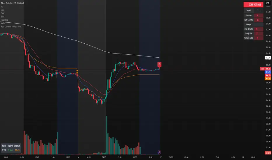
SJ Fx Session RangeSJ Fx Session Range Indicator
A Professional Forex Session Tracking Tool with Opening Range Analysis
Overview
The SJ Fx Session Range indicator is a comprehensive tool designed to help forex traders visualize major trading sessions (Asia, Europe+London, and New York) along with their first 15-minute opening ranges. Built with Pine Script v5, this indicator provides clear session boundaries, high/low ranges, and customizable opening range analysis to enhance your trading decisions.
Key Features
1. Trading Session Boxes
- Three major forex sessions: Asia, Europe+London, and New York
- Color-coded session boxes with transparent backgrounds for easy visualization
- Automatic session high/low tracking
- Session labels displayed inside boxes for quick identification
- Displays up to 50 historical sessions for pattern analysis
2. Opening Range Analysis
- Tracks first 15-minute opening range for Europe, London, and NY sessions
- Plots high, low, and mid-range levels
- Customizable line colors for each session's opening range
- Background highlights during the first 15 minutes of each session
- Helps identify potential breakout or reversal zones
3. Daylight Saving Time Support
- Built-in DST toggle for easy seasonal adjustment
- Automatically adjusts all session timings by 1 hour when enabled
- Clear tooltip instructions for when to enable/disable DST
- Default timings configured for IST timezone (Asia/Kolkata)
4. User-Friendly Design
- Clean input interface organized by session categories
- Fixed optimal settings for boxes and lines (50-day history)
- All session times are easily customizable with helpful tooltips
- Warning tooltips to prevent accidental timing changes
Default Session Times (when DST is disabled)
- Asia Session: 04:00 - 12:30 IST
- Europe + London Session: 12:30 - 20:00 IST
- New York Session: 20:00 - 02:30 IST
How to Use
1. Add to Chart: Apply the indicator to any forex pair chart
2. Adjust DST: Enable the "Start Daylight Saving Time Change" checkbox on the second Sunday in March; disable on the first Sunday in November
3. Customize Sessions: Toggle individual sessions on/off based on your trading preference
4. Opening Range Colors: Customize the opening range line colors for better visibility
5. Session Times: Default times are optimized for IST; modify only if trading from a different timezone
Technical Specifications
- Version: Pine Script v5
- Overlay: Yes (draws directly on price chart)
- Maximum Objects: 500 boxes, 500 lines
- History: 50 days of session data
- Timezone: Asia/Kolkata (IST) - customizable in code
Use Cases
- Identify high-liquidity trading periods
- Track session volatility patterns
- Monitor opening range breakouts/breakdowns
- Analyze session-specific price action
- Plan entries around major session opens
- Avoid trading during low-liquidity periods
Performance
Optimized for efficient rendering with:
- Fixed 50-day history limit for optimal performance
- Automatic cleanup of old session boxes and lines
- Lightweight code structure for fast chart loading
Customization Options
Available Inputs:
- Enable/disable individual sessions
- Adjust session timings (with safety tooltips)
- Toggle DST on/off
- Show/hide opening range analysis
- Customize opening range line colors for each session
Fixed for Optimal Performance:
- Session box colors (Asia: Aqua, Europe: Green, NY: Red)
- 50-day historical display
- Line width and style
- Mid-range line always displayed
Educational Value
This indicator helps traders:
- Understand forex market structure and session overlaps
- Recognize high-probability trading times
- Develop session-based trading strategies
- Improve timing of trade entries and exits
Open Source License
This script is published under Mozilla Public License 2.0, allowing you to:
- Use freely for personal trading
- Modify and adapt to your needs
- Learn from the code structure
- Share improvements with the community
Credits
Developed by Shantanu Joshi
- Designed for forex traders focusing on session-based strategies
- Built with clean, well-documented Pine Script v5 code
- Regular updates and improvements based on user feedback
Support & Feedback
If you find this indicator useful:
- Give it a thumbs up
- Share your trading results in the comments
- Suggest improvements or new features
- Report any issues for quick resolution
Disclaimer
This indicator is for educational and informational purposes only. It does not constitute financial advice. Always conduct your own research and risk management before making trading decisions. Past performance does not guarantee future results.
Compatible with: CFDs of forex pairs, commodities, indices, and crypto.
Best used on: 5-minutes
Recommended chart type: Candlestick charts

Lightning Session LevelsLightning Session Levels (LSL) draws clean, non-repainting levels for the major market sessions and a compact HUD in the top-right corner. It’s built to be lightweight, readable, and “set-and-forget” for intraday traders.
What it shows
Session High/Low and Open/Close levels for:
ASIA (00:00–08:00 UTC)
EUROPE (07:00–16:00 UTC)
US (13:30–20:00 UTC)
OVERNIGHT (20:00–24:00 UTC)
HUD panel:
Current active session
Countdown to the next US session (auto-calculated from UTC)
How it works (non-repainting)
Levels are anchored at session close. Each line is created once on the confirmed closing bar of the session (x2 = session end).
Optional Extend Right keeps the level projecting forward without changing the anchor (no “drifting”).
All drawings are pinned to the right price scale for stable reading.
Inputs
Show HUD — toggle the top-right panel.
Show Levels — master switch for drawing levels.
Draw High/Low — H/L session levels.
Draw Open/Close — O/C session levels.
Extend Right — extend all session lines to the future.
Keep N past sessions per market — FIFO limit per session group (default 12).
ASIA / EUROPE / US / OVERNIGHT — enable/disable specific sessions.
Style & palette
Consistent “Lightning” colors:
ASIA = Cyan, EUROPE = Violet, US = Amber, OVERNIGHT = Teal
Labels are always size: Normal for readability.
HUD uses a dark, subtle two-tone background to stay out of the way.
Recommended use
Timeframes: intraday (1m → 4h).
On 1D and higher, TradingView’s session-window time() filters won’t match intraday windows, so levels won’t plot (by design).
Markets: crypto, indices, FX, equities — any symbol where intraday session context helps.
Notes & limitations
Fixed UTC windows. The US window is set to 13:30–20:00 UTC. Daylight-saving shifts (DST) are not auto-adjusted; if you need region-specific DST behavior, treat this as a consistent UTC model.
The HUD timer counts down to the next US open from the current UTC clock.
Draw limits are capped (500 lines, 500 labels) for performance and stability.
Quick start
Add Lightning Session Levels to your chart.
Toggle Draw High/Low and/or Draw Open/Close.
Turn on Extend Right if you want the levels to project forward.
Enable only the sessions you care about (e.g., just EUROPE and US).
Use Keep N past sessions to control clutter (e.g., 6–12).
Disclaimer
This tool is for educational/informational purposes only and is not financial advice. Past session behavior does not guarantee future results. Always manage risk.

Volatility-Targeted Momentum Portfolio [BackQuant]Volatility-Targeted Momentum Portfolio
A complete momentum portfolio engine that ranks assets, targets a user-defined volatility, builds long, short, or delta-neutral books, and reports performance with metrics, attribution, Monte Carlo scenarios, allocation pie, and efficiency scatter plots. This description explains the theory and the mechanics so you can configure, validate, and deploy it with intent.
Table of contents
What the script does at a glance
Momentum, what it is, how to know if it is present
Volatility targeting, why and how it is done here
Portfolio construction modes: Long Only, Short Only, Delta Neutral
Regime filter and when the strategy goes to cash
Transaction cost modelling in this script
Backtest metrics and definitions
Performance attribution chart
Monte Carlo simulation
Scatter plot analysis modes
Asset allocation pie chart
Inputs, presets, and deployment checklist
Suggested workflow
1) What the script does at a glance
Pulls a list of up to 15 tickers, computes a simple momentum score on each over a configurable lookback, then volatility-scales their bar-to-bar return stream to a target annualized volatility.
Ranks assets by raw momentum, selects the top 3 and bottom 3, builds positions according to the chosen mode, and gates exposure with a fast regime filter.
Accumulates a portfolio equity curve with risk and performance metrics, optional benchmark buy-and-hold for comparison, and a full alert suite.
Adds visual diagnostics: performance attribution bars, Monte Carlo forward paths, an allocation pie, and scatter plots for risk-return and factor views.
2) Momentum: definition, detection, and validation
Momentum is the tendency of assets that have performed well to continue to perform well, and of underperformers to continue underperforming, over a specific horizon. You operationalize it by selecting a horizon, defining a signal, ranking assets, and trading the leaders versus laggards subject to risk constraints.
Signal choices . Common signals include cumulative return over a lookback window, regression slope on log-price, or normalized rate-of-change. This script uses cumulative return over lookback bars for ranking (variable cr = price/price - 1). It keeps the ranking simple and lets volatility targeting handle risk normalization.
How to know momentum is present .
Leaders and laggards persist across adjacent windows rather than flipping every bar.
Spread between average momentum of leaders and laggards is materially positive in sample.
Cross-sectional dispersion is non-trivial. If everything is flat or highly correlated with no separation, momentum selection will be weak.
Your validation should include a diagnostic that measures whether returns are explained by a momentum regression on the timeseries.
Recommended diagnostic tool . Before running any momentum portfolio, verify that a timeseries exhibits stable directional drift. Use this indicator as a pre-check: It fits a regression to price, exposes slope and goodness-of-fit style context, and helps confirm if there is usable momentum before you force a ranking into a flat regime.
3) Volatility targeting: purpose and implementation here
Purpose . Volatility targeting seeks a more stable risk footprint. High-vol assets get sized down, low-vol assets get sized up, so each contributes more evenly to total risk.
Computation in this script (per asset, rolling):
Return series ret = log(price/price ).
Annualized volatility estimate vol = stdev(ret, lookback) * sqrt(tradingdays).
Leverage multiplier volMult = clamp(targetVol / vol, 0.1, 5.0).
This caps sizing so extremely low-vol assets don’t explode weight and extremely high-vol assets don’t go to zero.
Scaled return stream sr = ret * volMult. This is the per-bar, risk-adjusted building block used in the portfolio combinations.
Interpretation . You are not levering your account on the exchange, you are rescaling the contribution each asset’s daily move has on the modeled equity. In live trading you would reflect this with position sizing or notional exposure.
4) Portfolio construction modes
Cross-sectional ranking . Assets are sorted by cr over the chosen lookback. Top and bottom indices are extracted without ties.
Long Only . Averages the volatility-scaled returns of the top 3 assets: avgRet = mean(sr_top1, sr_top2, sr_top3). Position table shows per-asset leverages and weights proportional to their current volMult.
Short Only . Averages the negative of the volatility-scaled returns of the bottom 3: avgRet = mean(-sr_bot1, -sr_bot2, -sr_bot3). Position table shows short legs.
Delta Neutral . Long the top 3 and short the bottom 3 in equal book sizes. Each side is sized to 50 percent notional internally, with weights within each side proportional to volMult. The return stream mixes the two sides: avgRet = mean(sr_top1,sr_top2,sr_top3, -sr_bot1,-sr_bot2,-sr_bot3).
Notes .
The selection metric is raw momentum, the execution stream is volatility-scaled returns. This separation is deliberate. It avoids letting volatility dominate ranking while still enforcing risk parity at the return contribution stage.
If everything rallies together and dispersion collapses, Long Only may behave like a single beta. Delta Neutral is designed to extract cross-sectional momentum with low net beta.
5) Regime filter
A fast EMA(12) vs EMA(21) filter gates exposure.
Long Only active when EMA12 > EMA21. Otherwise the book is set to cash.
Short Only active when EMA12 < EMA21. Otherwise cash.
Delta Neutral is always active.
This prevents taking long momentum entries during obvious local downtrends and vice versa for shorts. When the filter is false, equity is held flat for that bar.
6) Transaction cost modelling
There are two cost touchpoints in the script.
Per-bar drag . When the regime filter is active, the per-bar return is reduced by fee_rate * avgRet inside netRet = avgRet - (fee_rate * avgRet). This models proportional friction relative to traded impact on that bar.
Turnover-linked fee . The script tracks changes in membership of the top and bottom baskets (top1..top3, bot1..bot3). The intent is to charge fees when composition changes. The template counts changes and scales a fee by change count divided by 6 for the six slots.
Use case: increase fee_rate to reflect taker fees and slippage if you rebalance every bar or trade illiquid assets. Reduce it if you rebalance less often or use maker orders.
Practical advice .
If you rebalance daily, start with 5–20 bps round-trip per switch on liquid futures and adjust per venue.
For crypto perp microcaps, stress higher cost assumptions and add slippage buffers.
If you only rotate on lookback boundaries or at signals, use alert-driven rebalances and lower per-bar drag.
7) Backtest metrics and definitions
The script computes a standard set of portfolio statistics once the start date is reached.
Net Profit percent over the full test.
Max Drawdown percent, tracked from running peaks.
Annualized Mean and Stdev using the chosen trading day count.
Variance is the square of annualized stdev.
Sharpe uses daily mean adjusted by risk-free rate and annualized.
Sortino uses downside stdev only.
Omega ratio of sum of gains to sum of losses.
Gain-to-Pain total gains divided by total losses absolute.
CAGR compounded annual growth from start date to now.
Alpha, Beta versus a user-selected benchmark. Beta from covariance of daily returns, Alpha from CAPM.
Skewness of daily returns.
VaR 95 linear-interpolated 5th percentile of daily returns.
CVaR average of the worst 5 percent of daily returns.
Benchmark Buy-and-Hold equity path for comparison.
8) Performance attribution
Cumulative contribution per asset, adjusted for whether it was held long or short and for its volatility multiplier, aggregated across the backtest. You can filter to winners only or show both sides. The panel is sorted by contribution and includes percent labels.
9) Monte Carlo simulation
The panel draws forward equity paths from either a Normal model parameterized by recent mean and stdev, or non-parametric bootstrap of recent daily returns. You control the sample length, number of simulations, forecast horizon, visibility of individual paths, confidence bands, and a reproducible seed.
Normal uses Box-Muller with your seed. Good for quick, smooth envelopes.
Bootstrap resamples realized returns, preserving fat tails and volatility clustering better than a Gaussian assumption.
Bands show 10th, 25th, 75th, 90th percentiles and the path mean.
10) Scatter plot analysis
Four point-cloud modes, each plotting all assets and a star for the current portfolio position, with quadrant guides and labels.
Risk-Return Efficiency . X is risk proxy from leverage, Y is expected return from annualized momentum. The star shows the current book’s composite.
Momentum vs Volatility . Visualizes whether leaders are also high vol, a cue for turnover and cost expectations.
Beta vs Alpha . X is a beta proxy, Y is risk-adjusted excess return proxy. Useful to see if leaders are just beta.
Leverage vs Momentum . X is volMult, Y is momentum. Shows how volatility targeting is redistributing risk.
11) Asset allocation pie chart
Builds a wheel of current allocations.
Long Only, weights are proportional to each long asset’s current volMult and sum to 100 percent.
Short Only, weights show the short book as positive slices that sum to 100 percent.
Delta Neutral, 50 percent long and 50 percent short books, each side leverage-proportional.
Labels can show asset, percent, and current leverage.
12) Inputs and quick presets
Core
Portfolio Strategy . Long Only, Short Only, Delta Neutral.
Initial Capital . For equity scaling in the panel.
Trading Days/Year . 252 for stocks, 365 for crypto.
Target Volatility . Annualized, drives volMult.
Transaction Fees . Per-bar drag and composition change penalty, see the modelling notes above.
Momentum Lookback . Ranking horizon. Shorter is more reactive, longer is steadier.
Start Date . Ensure every symbol has data back to this date to avoid bias.
Benchmark . Used for alpha, beta, and B&H line.
Diagnostics
Metrics, Equity, B&H, Curve labels, Daily return line, Rolling drawdown fill.
Attribution panel. Toggle winners only to focus on what matters.
Monte Carlo mode with Normal or Bootstrap and confidence bands.
Scatter plot type and styling, labels, and portfolio star.
Pie chart and labels for current allocation.
Presets
Crypto Daily, Long Only . Lookback 25, Target Vol 50 percent, Fees 10 bps, Regime filter on, Metrics and Drawdown on. Monte Carlo Bootstrap with Recent 200 bars for bands.
Crypto Daily, Delta Neutral . Lookback 25, Target Vol 50 percent, Fees 15–25 bps, Regime filter always active for this mode. Use Scatter Risk-Return to monitor efficiency and keep the star near upper left quadrants without drifting rightward.
Equities Daily, Long Only . Lookback 60–120, Target Vol 15–20 percent, Fees 5–10 bps, Regime filter on. Use Benchmark SPX and watch Alpha and Beta to keep the book from becoming index beta.
13) Suggested workflow
Universe sanity check . Pick liquid tickers with stable data. Thin assets distort vol estimates and fees.
Check momentum existence . Run on your timeframe. If slope and fit are weak, widen lookback or avoid that asset or timeframe.
Set risk budget . Choose a target volatility that matches your drawdown tolerance. Higher target increases turnover and cost sensitivity.
Pick mode . Long Only for bull regimes, Short Only for sustained downtrends, Delta Neutral for cross-sectional harvesting when index direction is unclear.
Tune lookback . If leaders rotate too often, lengthen it. If entries lag, shorten it.
Validate cost assumptions . Increase fee_rate and stress Monte Carlo. If the edge vanishes with modest friction, refine selection or lengthen rebalance cadence.
Run attribution . Confirm the strategy’s winners align with intuition and not one unstable outlier.
Use alerts . Enable position change, drawdown, volatility breach, regime, momentum shift, and crash alerts to supervise live runs.
Important implementation details mapped to code
Momentum measure . cr = price / price - 1 per symbol for ranking. Simplicity helps avoid overfitting.
Volatility targeting . vol = stdev(log returns, lookback) * sqrt(tradingdays), volMult = clamp(targetVol / vol, 0.1, 5), sr = ret * volMult.
Selection . Extract indices for top1..top3 and bot1..bot3. The arrays rets, scRets, lev_vals, and ticks_arr track momentum, scaled returns, leverage multipliers, and display tickers respectively.
Regime filter . EMA12 vs EMA21 switch determines if the strategy takes risk for Long or Short modes. Delta Neutral ignores the gate.
Equity update . Equity multiplies by 1 + netRet only when the regime was active in the prior bar. Buy-and-hold benchmark is computed separately for comparison.
Tables . Position tables show current top or bottom assets with leverage and weights. Metric table prints all risk and performance figures.
Visualization panels . Attribution, Monte Carlo, scatter, and pie use the last bars to draw overlays that update as the backtest proceeds.
Final notes
Momentum is a portfolio effect. The edge comes from cross-sectional dispersion, adequate risk normalization, and disciplined turnover control, not from a single best asset call.
Volatility targeting stabilizes path but does not fix selection. Use the momentum regression link above to confirm structure exists before you size into it.
Always test higher lag costs and slippage, then recheck metrics, attribution, and Monte Carlo envelopes. If the edge persists under stress, you have something robust.

Algorithm Predator - ML-liteAlgorithm Predator - ML-lite
This indicator combines four specialized trading agents with an adaptive multi-armed bandit selection system to identify high-probability trade setups. It is designed for swing and intraday traders who want systematic signal generation based on institutional order flow patterns , momentum exhaustion , liquidity dynamics , and statistical mean reversion .
Core Architecture
Why These Components Are Combined:
The script addresses a fundamental challenge in algorithmic trading: no single detection method works consistently across all market conditions. By deploying four independent agents and using reinforcement learning algorithms to select or blend their outputs, the system adapts to changing market regimes without manual intervention.
The Four Trading Agents
1. Spoofing Detector Agent 🎭
Detects iceberg orders through persistent volume at similar price levels over 5 bars
Identifies spoofing patterns via asymmetric wick analysis (wicks exceeding 60% of bar range with volume >1.8× average)
Monitors order clustering using simplified Hawkes process intensity tracking (exponential decay model)
Signal Logic: Contrarian—fades false breakouts caused by institutional manipulation
Best Markets: Consolidations, institutional trading windows, low-liquidity hours
2. Exhaustion Detector Agent ⚡
Calculates RSI divergence between price movement and momentum indicator over 5-bar window
Detects VWAP exhaustion (price at 2σ bands with declining volume)
Uses VPIN reversals (volume-based toxic flow dissipation) to identify momentum failure
Signal Logic: Counter-trend—enters when momentum extreme shows weakness
Best Markets: Trending markets reaching climax points, over-extended moves
3. Liquidity Void Detector Agent 💧
Measures Bollinger Band squeeze (width <60% of 50-period average)
Identifies stop hunts via 20-bar high/low penetration with immediate reversal and volume spike
Detects hidden liquidity absorption (volume >2× average with range <0.3× ATR)
Signal Logic: Breakout anticipation—enters after liquidity grab but before main move
Best Markets: Range-bound pre-breakout, volatility compression zones
4. Mean Reversion Agent 📊
Calculates price z-scores relative to 50-period SMA and standard deviation (triggers at ±2σ)
Implements Ornstein-Uhlenbeck process scoring (mean-reverting stochastic model)
Uses entropy analysis to detect algorithmic trading patterns (low entropy <0.25 = high predictability)
Signal Logic: Statistical reversion—enters when price deviates significantly from statistical equilibrium
Best Markets: Range-bound, low-volatility, algorithmically-dominated instruments
Adaptive Selection: Multi-Armed Bandit System
The script implements four reinforcement learning algorithms to dynamically select or blend agents based on performance:
Thompson Sampling (Default - Recommended):
Uses Bayesian inference with beta distributions (tracks alpha/beta parameters per agent)
Balances exploration (trying underused agents) vs. exploitation (using proven winners)
Each agent's win/loss history informs its selection probability
Lite Approximation: Uses pseudo-random sampling from price/volume noise instead of true random number generation
UCB1 (Upper Confidence Bound):
Calculates confidence intervals using: average_reward + sqrt(2 × ln(total_pulls) / agent_pulls)
Deterministic algorithm favoring agents with high uncertainty (potential upside)
More conservative than Thompson Sampling
Epsilon-Greedy:
Exploits best-performing agent (1-ε)% of the time
Explores randomly ε% of the time (default 10%, configurable 1-50%)
Simple, transparent, easily tuned via epsilon parameter
Gradient Bandit:
Uses softmax probability distribution over agent preference weights
Updates weights via gradient ascent based on rewards
Best for Blend mode where all agents contribute
Selection Modes:
Switch Mode: Uses only the selected agent's signal (clean, decisive)
Blend Mode: Combines all agents using exponentially weighted confidence scores controlled by temperature parameter (smooth, diversified)
Lock Agent Feature:
Optional manual override to force one specific agent
Useful after identifying which agent dominates your specific instrument
Only applies in Switch mode
Four choices: Spoofing Detector, Exhaustion Detector, Liquidity Void, Mean Reversion
Memory System
Dual-Layer Architecture:
Short-Term Memory: Stores last 20 trade outcomes per agent (configurable 10-50)
Long-Term Memory: Stores episode averages when short-term reaches transfer threshold (configurable 5-20 bars)
Memory Boost Mechanism: Recent performance modulates agent scores by up to ±20%
Episode Transfer: When an agent accumulates sufficient results, averages are condensed into long-term storage
Persistence: Manual restoration of learned parameters via input fields (alpha, beta, weights, microstructure thresholds)
How Memory Works:
Agent generates signal → outcome tracked after 8 bars (performance horizon)
Result stored in short-term memory (win = 1.0, loss = 0.0)
Short-term average influences agent's future scores (positive feedback loop)
After threshold met (default 10 results), episode averaged into long-term storage
Long-term patterns (weighted 30%) + short-term patterns (weighted 70%) = total memory boost
Market Microstructure Analysis
These advanced metrics quantify institutional order flow dynamics:
Order Flow Toxicity (Simplified VPIN):
Measures buy/sell volume imbalance over 20 bars: |buy_vol - sell_vol| / (buy_vol + sell_vol)
Detects informed trading activity (institutional players with non-public information)
Values >0.4 indicate "toxic flow" (informed traders active)
Lite Approximation: Uses simple open/close heuristic instead of tick-by-tick trade classification
Price Impact Analysis (Simplified Kyle's Lambda):
Measures market impact efficiency: |price_change_10| / sqrt(volume_sum_10)
Low values = large orders with minimal price impact ( stealth accumulation )
High values = retail-dominated moves with high slippage
Lite Approximation: Uses simplified denominator instead of regression-based signed order flow
Market Randomness (Entropy Analysis):
Counts unique price changes over 20 bars / 20
Measures market predictability
High entropy (>0.6) = human-driven, chaotic price action
Low entropy (<0.25) = algorithmic trading dominance (predictable patterns)
Lite Approximation: Simple ratio instead of true Shannon entropy H(X) = -Σ p(x)·log₂(p(x))
Order Clustering (Simplified Hawkes Process):
Tracks self-exciting event intensity (coordinated order activity)
Decays at 0.9× per bar, spikes +1.0 when volume >1.5× average
High intensity (>0.7) indicates clustering (potential spoofing/accumulation)
Lite Approximation: Simple exponential decay instead of full λ(t) = μ + Σ α·exp(-β(t-tᵢ)) with MLE
Signal Generation Process
Multi-Stage Validation:
Stage 1: Agent Scoring
Each agent calculates internal score based on its detection criteria
Scores must exceed agent-specific threshold (adjusted by sensitivity multiplier)
Agent outputs: Signal direction (+1/-1/0) and Confidence level (0.0-1.0)
Stage 2: Memory Boost
Agent scores multiplied by memory boost factor (0.8-1.2 based on recent performance)
Successful agents get amplified, failing agents get dampened
Stage 3: Bandit Selection/Blending
If Adaptive Mode ON:
Switch: Bandit selects single best agent, uses only its signal
Blend: All agents combined using softmax-weighted confidence scores
If Adaptive Mode OFF:
Traditional consensus voting with confidence-squared weighting
Signal fires when consensus exceeds threshold (default 70%)
Stage 4: Confirmation Filter
Raw signal must repeat for consecutive bars (default 3, configurable 2-4)
Minimum confidence threshold: 0.25 (25%) enforced regardless of mode
Trend alignment check: Long signals require trend_score ≥ -2, Short signals require trend_score ≤ 2
Stage 5: Cooldown Enforcement
Minimum bars between signals (default 10, configurable 5-15)
Prevents over-trading during choppy conditions
Stage 6: Performance Tracking
After 8 bars (performance horizon), signal outcome evaluated
Win = price moved in signal direction, Loss = price moved against
Results fed back into memory and bandit statistics
Trading Modes (Presets)
Pre-configured parameter sets:
Conservative: 85% consensus, 4 confirmations, 15-bar cooldown
Expected: 60-70% win rate, 3-8 signals/week
Best for: Swing trading, capital preservation, beginners
Balanced: 70% consensus, 3 confirmations, 10-bar cooldown
Expected: 55-65% win rate, 8-15 signals/week
Best for: Day trading, most traders, general use
Aggressive: 60% consensus, 2 confirmations, 5-bar cooldown
Expected: 50-58% win rate, 15-30 signals/week
Best for: Scalping, high-frequency trading, active management
Elite: 75% consensus, 3 confirmations, 12-bar cooldown
Expected: 58-68% win rate, 5-12 signals/week
Best for: Selective trading, high-conviction setups
Adaptive: 65% consensus, 2 confirmations, 8-bar cooldown
Expected: Varies based on learning
Best for: Experienced users leveraging bandit system
How to Use
1. Initial Setup (5 Minutes):
Select Trading Mode matching your style (start with Balanced)
Enable Adaptive Learning (recommended for automatic agent selection)
Choose Thompson Sampling algorithm (best all-around performance)
Keep Microstructure Metrics enabled for liquid instruments (>100k daily volume)
2. Agent Tuning (Optional):
Adjust Agent Sensitivity multipliers (0.5-2.0):
<0.8 = Highly selective (fewer signals, higher quality)
0.9-1.2 = Balanced (recommended starting point)
1.3 = Aggressive (more signals, lower individual quality)
Monitor dashboard for 20-30 signals to identify dominant agent
If one agent consistently outperforms, consider using Lock Agent feature
3. Bandit Configuration (Advanced):
Blend Temperature (0.1-2.0):
0.3 = Sharp decisions (best agent dominates)
0.5 = Balanced (default)
1.0+ = Smooth (equal weighting, democratic)
Memory Decay (0.8-0.99):
0.90 = Fast adaptation (volatile markets)
0.95 = Balanced (most instruments)
0.97+ = Long memory (stable trends)
4. Signal Interpretation:
Green triangle (▲): Long signal confirmed
Red triangle (▼): Short signal confirmed
Dashboard shows:
Active agent (highlighted row with ► marker)
Win rate per agent (green >60%, yellow 40-60%, red <40%)
Confidence bars (█████ = maximum confidence)
Memory size (short-term buffer count)
Colored zones display:
Entry level (current close)
Stop-loss (1.5× ATR)
Take-profit 1 (2.0× ATR)
Take-profit 2 (3.5× ATR)
5. Risk Management:
Never risk >1-2% per signal (use ATR-based stops)
Signals are entry triggers, not complete strategies
Combine with your own market context analysis
Consider fundamental catalysts and news events
Use "Confirming" status to prepare entries (not to enter early)
6. Memory Persistence (Optional):
After 50-100 trades, check Memory Export Panel
Record displayed alpha/beta/weight values for each agent
Record VPIN and Kyle threshold values
Enable "Restore From Memory" and input saved values to continue learning
Useful when switching timeframes or restarting indicator
Visual Components
On-Chart Elements:
Spectral Layers: EMA8 ± 0.5 ATR bands (dynamic support/resistance, colored by trend)
Energy Radiance: Multi-layer glow boxes at signal points (intensity scales with confidence, configurable 1-5 layers)
Probability Cones: Projected price paths with uncertainty wedges (15-bar projection, width = confidence × ATR)
Connection Lines: Links sequential signals (solid = same direction continuation, dotted = reversal)
Kill Zones: Risk/reward boxes showing entry, stop-loss, and dual take-profit targets
Signal Markers: Triangle up/down at validated entry points
Dashboard (Configurable Position & Size):
Regime Indicator: 4-level trend classification (Strong Bull/Bear, Weak Bull/Bear)
Mode Status: Shows active system (Adaptive Blend, Locked Agent, or Consensus)
Agent Performance Table: Real-time win%, confidence, and memory stats
Order Flow Metrics: Toxicity and impact indicators (when microstructure enabled)
Signal Status: Current state (Long/Short/Confirming/Waiting) with confirmation progress
Memory Panel (Configurable Position & Size):
Live Parameter Export: Alpha, beta, and weight values per agent
Adaptive Thresholds: Current VPIN sensitivity and Kyle threshold
Save Reminder: Visual indicator if parameters should be recorded
What Makes This Original
This script's originality lies in three key innovations:
1. Genuine Meta-Learning Framework:
Unlike traditional indicator mashups that simply display multiple signals, this implements authentic reinforcement learning (multi-armed bandits) to learn which detection method works best in current conditions. The Thompson Sampling implementation with beta distribution tracking (alpha for successes, beta for failures) is statistically rigorous and adapts continuously. This is not post-hoc optimization—it's real-time learning.
2. Episodic Memory Architecture with Transfer Learning:
The dual-layer memory system mimics human learning patterns:
Short-term memory captures recent performance (recency bias)
Long-term memory preserves historical patterns (experience)
Automatic transfer mechanism consolidates knowledge
Memory boost creates positive feedback loops (successful strategies become stronger)
This architecture allows the system to adapt without retraining , unlike static ML models that require batch updates.
3. Institutional Microstructure Integration:
Combines retail-focused technical analysis (RSI, Bollinger Bands, VWAP) with institutional-grade microstructure metrics (VPIN, Kyle's Lambda, Hawkes processes) typically found in academic finance literature and professional trading systems, not standard retail platforms. While simplified for Pine Script constraints, these metrics provide insight into informed vs. uninformed trading , a dimension entirely absent from traditional technical analysis.
Mashup Justification:
The four agents are combined specifically for risk diversification across failure modes:
Spoofing Detector: Prevents false breakout losses from manipulation
Exhaustion Detector: Prevents chasing extended trends into reversals
Liquidity Void: Exploits volatility compression (different regime than trending)
Mean Reversion: Provides mathematical anchoring when patterns fail
The bandit system ensures the optimal tool is automatically selected for each market situation, rather than requiring manual interpretation of conflicting signals.
Why "ML-lite"? Simplifications and Approximations
This is the "lite" version due to necessary simplifications for Pine Script execution:
1. Simplified VPIN Calculation:
Academic Implementation: True VPIN uses volume bucketing (fixed-volume bars) and tick-by-tick buy/sell classification via Lee-Ready algorithm or exchange-provided trade direction flags
This Implementation: 20-bar rolling window with simple open/close heuristic (close > open = buy volume)
Impact: May misclassify volume during ranging/choppy markets; works best in directional moves
2. Pseudo-Random Sampling:
Academic Implementation: Thompson Sampling requires true random number generation from beta distributions using inverse transform sampling or acceptance-rejection methods
This Implementation: Deterministic pseudo-randomness derived from price and volume decimal digits: (close × 100 - floor(close × 100)) + (volume % 100) / 100
Impact: Not cryptographically random; may have subtle biases in specific price ranges; provides sufficient variation for agent selection
3. Hawkes Process Approximation:
Academic Implementation: Full Hawkes process uses maximum likelihood estimation with exponential kernels: λ(t) = μ + Σ α·exp(-β(t-tᵢ)) fitted via iterative optimization
This Implementation: Simple exponential decay (0.9 multiplier) with binary event triggers (volume spike = event)
Impact: Captures self-exciting property but lacks parameter optimization; fixed decay rate may not suit all instruments
4. Kyle's Lambda Simplification:
Academic Implementation: Estimated via regression of price impact on signed order flow over multiple time intervals: Δp = λ × Δv + ε
This Implementation: Simplified ratio: price_change / sqrt(volume_sum) without proper signed order flow or regression
Impact: Provides directional indicator of impact but not true market depth measurement; no statistical confidence intervals
5. Entropy Calculation:
Academic Implementation: True Shannon entropy requires probability distribution: H(X) = -Σ p(x)·log₂(p(x)) where p(x) is probability of each price change magnitude
This Implementation: Simple ratio of unique price changes to total observations (variety measure)
Impact: Measures diversity but not true information entropy with probability weighting; less sensitive to distribution shape
6. Memory System Constraints:
Full ML Implementation: Neural networks with backpropagation, experience replay buffers (storing state-action-reward tuples), gradient descent optimization, and eligibility traces
This Implementation: Fixed-size array queues with simple averaging; no gradient-based learning, no state representation beyond raw scores
Impact: Cannot learn complex non-linear patterns; limited to linear performance tracking
7. Limited Feature Engineering:
Advanced Implementation: Dozens of engineered features, polynomial interactions (x², x³), dimensionality reduction (PCA, autoencoders), feature selection algorithms
This Implementation: Raw agent scores and basic market metrics (RSI, ATR, volume ratio); minimal transformation
Impact: May miss subtle cross-feature interactions; relies on agent-level intelligence rather than feature combinations
8. Single-Instrument Data:
Full Implementation: Multi-asset correlation analysis (sector ETFs, currency pairs, volatility indices like VIX), lead-lag relationships, risk-on/risk-off regimes
This Implementation: Only OHLCV data from displayed instrument
Impact: Cannot incorporate broader market context; vulnerable to correlated moves across assets
9. Fixed Performance Horizon:
Full Implementation: Adaptive horizon based on trade duration, volatility regime, or profit target achievement
This Implementation: Fixed 8-bar evaluation window
Impact: May evaluate too early in slow markets or too late in fast markets; one-size-fits-all approach
Performance Impact Summary:
These simplifications make the script:
✅ Faster: Executes in milliseconds vs. seconds (or minutes) for full academic implementations
✅ More Accessible: Runs on any TradingView plan without external data feeds, APIs, or compute servers
✅ More Transparent: All calculations visible in Pine Script (no black-box compiled models)
✅ Lower Resource Usage: <500 bars lookback, minimal memory footprint
⚠️ Less Precise: Approximations may reduce statistical edge by 5-15% vs. academic implementations
⚠️ Limited Scope: Cannot capture tick-level dynamics, multi-order-book interactions, or cross-asset flows
⚠️ Fixed Parameters: Some thresholds hardcoded rather than dynamically optimized
When to Upgrade to Full Implementation:
Consider professional Python/C++ versions with institutional data feeds if:
Trading with >$100K capital where precision differences materially impact returns
Operating in microsecond-competitive environments (HFT, market making)
Requiring regulatory-grade audit trails and reproducibility
Backtesting with tick-level precision for strategy validation
Need true real-time adaptation with neural network-based learning
For retail swing/day trading and position management, these approximations provide sufficient signal quality while maintaining usability, transparency, and accessibility. The core logic—multi-agent detection with adaptive selection—remains intact.
Technical Notes
All calculations use standard Pine Script built-in functions ( ta.ema, ta.atr, ta.rsi, ta.bb, ta.sma, ta.stdev, ta.vwap )
VPIN and Kyle's Lambda use simplified formulas optimized for OHLCV data (see "Lite" section above)
Thompson Sampling uses pseudo-random noise from price/volume decimal digits for beta distribution sampling
No repainting: All calculations use confirmed bar data (no forward-looking)
Maximum lookback: 500 bars (set via max_bars_back parameter)
Performance evaluation: 8-bar forward-looking window for reward calculation (clearly disclosed)
Confidence threshold: Minimum 0.25 (25%) enforced on all signals
Memory arrays: Dynamic sizing with FIFO queue management
Limitations and Disclaimers
Not Predictive: This indicator identifies patterns in historical data. It cannot predict future price movements with certainty.
Requires Human Judgment: Signals are entry triggers, not complete trading strategies. Must be confirmed with your own analysis, risk management rules, and market context.
Learning Period Required: The adaptive system requires 50-100 bars minimum to build statistically meaningful performance data for bandit algorithms.
Overfitting Risk: Restoring memory parameters from one market regime to a drastically different regime (e.g., low volatility to high volatility) may cause poor initial performance until system re-adapts.
Approximation Limitations: Simplified calculations (see "Lite" section) may underperform academic implementations by 5-15% in highly efficient markets.
No Guarantee of Profit: Past performance, whether backtested or live-traded, does not guarantee future performance. All trading involves risk of loss.
Forward-Looking Bias: Performance evaluation uses 8-bar forward window—this creates slight look-ahead for learning (though not for signals). Real-time performance may differ from indicator's internal statistics.
Single-Instrument Limitation: Does not account for correlations with related assets or broader market regime changes.
Recommended Settings
Timeframe: 15-minute to 4-hour charts (sufficient volatility for ATR-based stops; adequate bar volume for learning)
Assets: Liquid instruments with >100k daily volume (forex majors, large-cap stocks, BTC/ETH, major indices)
Not Recommended: Illiquid small-caps, penny stocks, low-volume altcoins (microstructure metrics unreliable)
Complementary Tools: Volume profile, order book depth, market breadth indicators, fundamental catalysts
Position Sizing: Risk no more than 1-2% of capital per signal using ATR-based stop-loss
Signal Filtering: Consider external confluence (support/resistance, trendlines, round numbers, session opens)
Start With: Balanced mode, Thompson Sampling, Blend mode, default agent sensitivities (1.0)
After 30+ Signals: Review agent win rates, consider increasing sensitivity of top performers or locking to dominant agent
Alert Configuration
The script includes built-in alert conditions:
Long Signal: Fires when validated long entry confirmed
Short Signal: Fires when validated short entry confirmed
Alerts fire once per bar (after confirmation requirements met)
Set alert to "Once Per Bar Close" for reliability
Taking you to school. — Dskyz, Trade with insight. Trade with anticipation.
