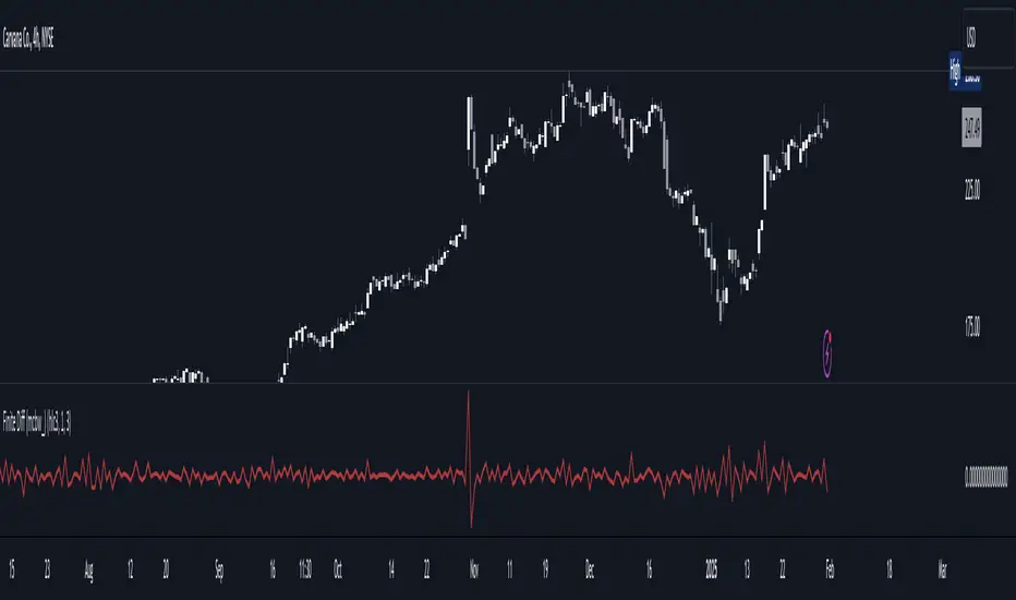
Finite Difference - Backward (mcbw_)In calculus there exists a 'derivative', which simply just measures the difference between two points on a curve. For well behaved mathematical functions there are infinitely many points and so there exists a derivative at every point. Where there are infinitely many points in a curve that curve is called 'continuous'. Continuous curves are very nice to deal with since each point on it exists almost exactly where its neighbors are. However, if the curve does not have infinitely many points on it, but instead has a finite number of points on it, that curve is called 'discrete' instead of continuous. Taking the derivative of discrete curves is much trickier business since there are none of the mathematical conveniences that a continuous offers. In the real world everything we measure is a discrete curve, including Price (since we measure it a finite number of times, aka each candlestick)!
The branch of Discrete Mathematics has found an approach to measure the derivative along a discrete curve, that approach is aptly called " Finite Difference ". To get a more accurate approximation of a discrete derivative, the finite difference approach uses weighted combinations of neighboring points. The most common type of finite difference is a 'central' difference, this uses a combination of points before and after the point of interest to approximate the discrete derivative. This is great for historical analysis but is not of much use for trading algorithms since it technically means using future prices to calculate the derivative of the current point. Instead we can use a less common variant called a ' Backwards Difference ' that only uses a combination of points before the current one to help approximate the current derivative.
In this script you can choose the " Order " of your derivative and the " Accuracy " of its approximation. This script is for educational purposes for folks building trading algorithms. Many trading algorithms often have an element of seeing how much Price has changed from the previous candle to the current candle. This approach is the lowest accuracy derivative possible, and using the backwards finite differences, made available for the first time on TradingView (!!), algorithms that use derivatives can now have higher orders of accuracy!
Happy Trading/Developing!
Backward
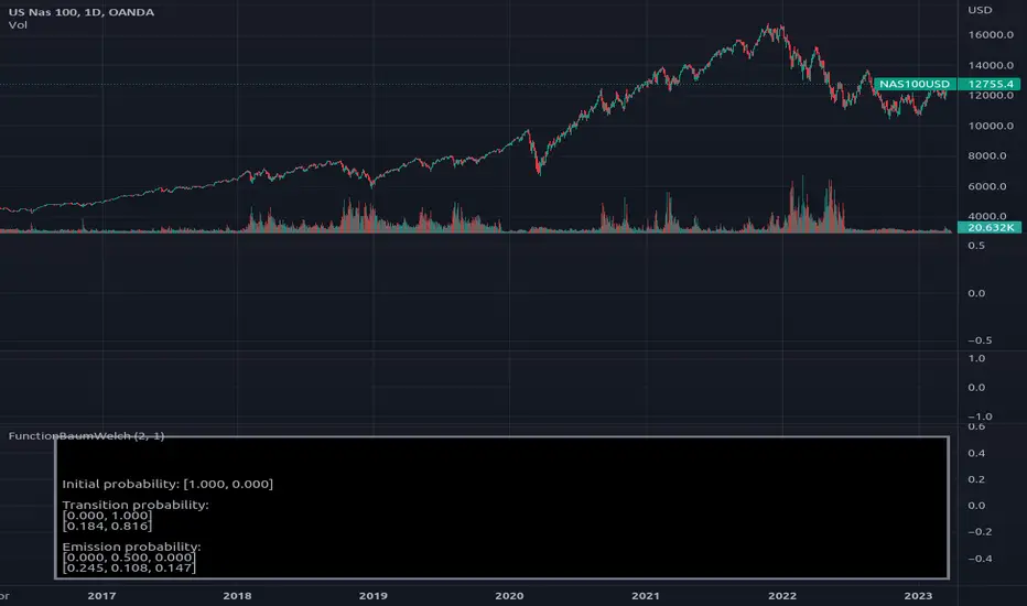
FunctionBaumWelchLibrary "FunctionBaumWelch"
Baum-Welch Algorithm, also known as Forward-Backward Algorithm, uses the well known EM algorithm
to find the maximum likelihood estimate of the parameters of a hidden Markov model given a set of observed
feature vectors.
---
### Function List:
> `forward (array pi, matrix a, matrix b, array obs)`
> `forward (array pi, matrix a, matrix b, array obs, bool scaling)`
> `backward (matrix a, matrix b, array obs)`
> `backward (matrix a, matrix b, array obs, array c)`
> `baumwelch (array observations, int nstates)`
> `baumwelch (array observations, array pi, matrix a, matrix b)`
---
### Reference:
> en.wikipedia.org
> github.com
> en.wikipedia.org
> www.rdocumentation.org
> www.rdocumentation.org
forward(pi, a, b, obs)
Computes forward probabilities for state `X` up to observation at time `k`, is defined as the
probability of observing sequence of observations `e_1 ... e_k` and that the state at time `k` is `X`.
Parameters:
pi (float ) : Initial probabilities.
a (matrix) : Transmissions, hidden transition matrix a or alpha = transition probability matrix of changing
states given a state matrix is size (M x M) where M is number of states.
b (matrix) : Emissions, matrix of observation probabilities b or beta = observation probabilities. Given
state matrix is size (M x O) where M is number of states and O is number of different
possible observations.
obs (int ) : List with actual state observation data.
Returns: - `matrix _alpha`: Forward probabilities. The probabilities are given on a logarithmic scale (natural logarithm). The first
dimension refers to the state and the second dimension to time.
forward(pi, a, b, obs, scaling)
Computes forward probabilities for state `X` up to observation at time `k`, is defined as the
probability of observing sequence of observations `e_1 ... e_k` and that the state at time `k` is `X`.
Parameters:
pi (float ) : Initial probabilities.
a (matrix) : Transmissions, hidden transition matrix a or alpha = transition probability matrix of changing
states given a state matrix is size (M x M) where M is number of states.
b (matrix) : Emissions, matrix of observation probabilities b or beta = observation probabilities. Given
state matrix is size (M x O) where M is number of states and O is number of different
possible observations.
obs (int ) : List with actual state observation data.
scaling (bool) : Normalize `alpha` scale.
Returns: - #### Tuple with:
> - `matrix _alpha`: Forward probabilities. The probabilities are given on a logarithmic scale (natural logarithm). The first
dimension refers to the state and the second dimension to time.
> - `array _c`: Array with normalization scale.
backward(a, b, obs)
Computes backward probabilities for state `X` and observation at time `k`, is defined as the probability of observing the sequence of observations `e_k+1, ... , e_n` under the condition that the state at time `k` is `X`.
Parameters:
a (matrix) : Transmissions, hidden transition matrix a or alpha = transition probability matrix of changing states
given a state matrix is size (M x M) where M is number of states
b (matrix) : Emissions, matrix of observation probabilities b or beta = observation probabilities. given state
matrix is size (M x O) where M is number of states and O is number of different possible observations
obs (int ) : Array with actual state observation data.
Returns: - `matrix _beta`: Backward probabilities. The probabilities are given on a logarithmic scale (natural logarithm). The first dimension refers to the state and the second dimension to time.
backward(a, b, obs, c)
Computes backward probabilities for state `X` and observation at time `k`, is defined as the probability of observing the sequence of observations `e_k+1, ... , e_n` under the condition that the state at time `k` is `X`.
Parameters:
a (matrix) : Transmissions, hidden transition matrix a or alpha = transition probability matrix of changing states
given a state matrix is size (M x M) where M is number of states
b (matrix) : Emissions, matrix of observation probabilities b or beta = observation probabilities. given state
matrix is size (M x O) where M is number of states and O is number of different possible observations
obs (int ) : Array with actual state observation data.
c (float ) : Array with Normalization scaling coefficients.
Returns: - `matrix _beta`: Backward probabilities. The probabilities are given on a logarithmic scale (natural logarithm). The first dimension refers to the state and the second dimension to time.
baumwelch(observations, nstates)
**(Random Initialization)** Baum–Welch algorithm is a special case of the expectation–maximization algorithm used to find the
unknown parameters of a hidden Markov model (HMM). It makes use of the forward-backward algorithm
to compute the statistics for the expectation step.
Parameters:
observations (int ) : List of observed states.
nstates (int)
Returns: - #### Tuple with:
> - `array _pi`: Initial probability distribution.
> - `matrix _a`: Transition probability matrix.
> - `matrix _b`: Emission probability matrix.
---
requires: `import RicardoSantos/WIPTensor/2 as Tensor`
baumwelch(observations, pi, a, b)
Baum–Welch algorithm is a special case of the expectation–maximization algorithm used to find the
unknown parameters of a hidden Markov model (HMM). It makes use of the forward-backward algorithm
to compute the statistics for the expectation step.
Parameters:
observations (int ) : List of observed states.
pi (float ) : Initial probaility distribution.
a (matrix) : Transmissions, hidden transition matrix a or alpha = transition probability matrix of changing states
given a state matrix is size (M x M) where M is number of states
b (matrix) : Emissions, matrix of observation probabilities b or beta = observation probabilities. given state
matrix is size (M x O) where M is number of states and O is number of different possible observations
Returns: - #### Tuple with:
> - `array _pi`: Initial probability distribution.
> - `matrix _a`: Transition probability matrix.
> - `matrix _b`: Emission probability matrix.
---
requires: `import RicardoSantos/WIPTensor/2 as Tensor`
Backward Number of BarsThis indicator was written in order to apply bar limit in strategies and it was published as open code so that everyone can use it. When backtesting with stock market api data, we determine how many bars should be, not from which date the data will be drawn. For example, we can draw 1000 bar data from stock exchange and perform the backtest on this data. You can plan your strategy by checking the number of bars you test with the window () == 1 parameter here while checking through Tradingview to check that the test we performed gives correct results.
